P.S. Looking for the code for this? Available on github: recsys-nlp-graph

In the previous post, we established that a baseline recommender system (“recsys”) based on matrix factorization is able to achieve an AUC-ROC of ~0.8 (random guessing has AUC-ROC = 0.5)

Can we do better? Also, for curiosity’s sake, are there other approaches to recsys?

As it turns out, yes, and yes.

Natural Language Processing (NLP) and Graphs

In 2013, a breakthrough was made in NLP with the word2vec papers by Tomas Mikolov here and here. They demonstrated that w2v was able to learn semantic and syntactic vector representations of words in an unsupervised fashion.

Simply put, w2v can convert words (or objects) in sequences into a numeric representation, without labels—not needing labels is huge as getting labelled data is a key bottleneck in machine learning.

Another interesting development is DeepWalk which learns representations of online social networks graphs. By performing random walks to generate sequences, the paper demonstrated that it was able to learn vector representations of nodes (e.g., profiles, content) in the graph.

Figure 1a. Arbitrary image of a (social) graph

How do these matter in recsys?

It’s a slight stretch, but here’s the gist of it:

• Use the product-pairs and associated relationships to create a graph
• Generate sequences from the graph (via random walk)
• Learn product embeddings based on the sequences (via word2vec)
• Recommend products based on embedding similarity (e.g., cosine similarity, dot product)

Ready? Let’s get started.

Creating a graph

We have product-pairs and each of them have an associated score. We can think of them as (graph) edge weights.

With these weights, we can create a weighted graph (i.e., a graph where each edge is given a numerical weight, instead of all edges having the same weight). This can be easily done with networkx.

Violà! We have our product network graph.

Generating sequences

With our product graph, we can generate sequences via random walk.

The direct approach is to traverse the networkx graph. For example, if we want 10 sequences of length 10 for each starting node, we’ll need to traverse the graph 100 times per starting node (also called vertex).

The electronics graph has 420k nodes and the books graph has 2 million nodes. Multiply that by 100 and that’s a lot of graph queries—this is very slow and takes a lot of memory (trust me).

Thankfully, we don’t need to traverse the graph using the networkx APIs.

Using the transition matrix

A graph consists of vertices and edges, where edges are the strength of relationships between each node.

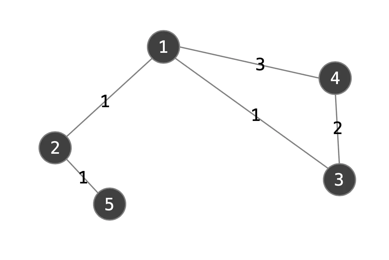
Figure 1b. Example weighted graph

This can be decomposed into an adjacency matrix. If our graph has V nodes, then our adjacency matrix will be V x V in dimension. A regular adjacency matrix has a value of 1 if an edge exists between the nodes, 0 otherwise. Since the graph edges are weighted, the values in the adjacency matrix will be the edge weights.

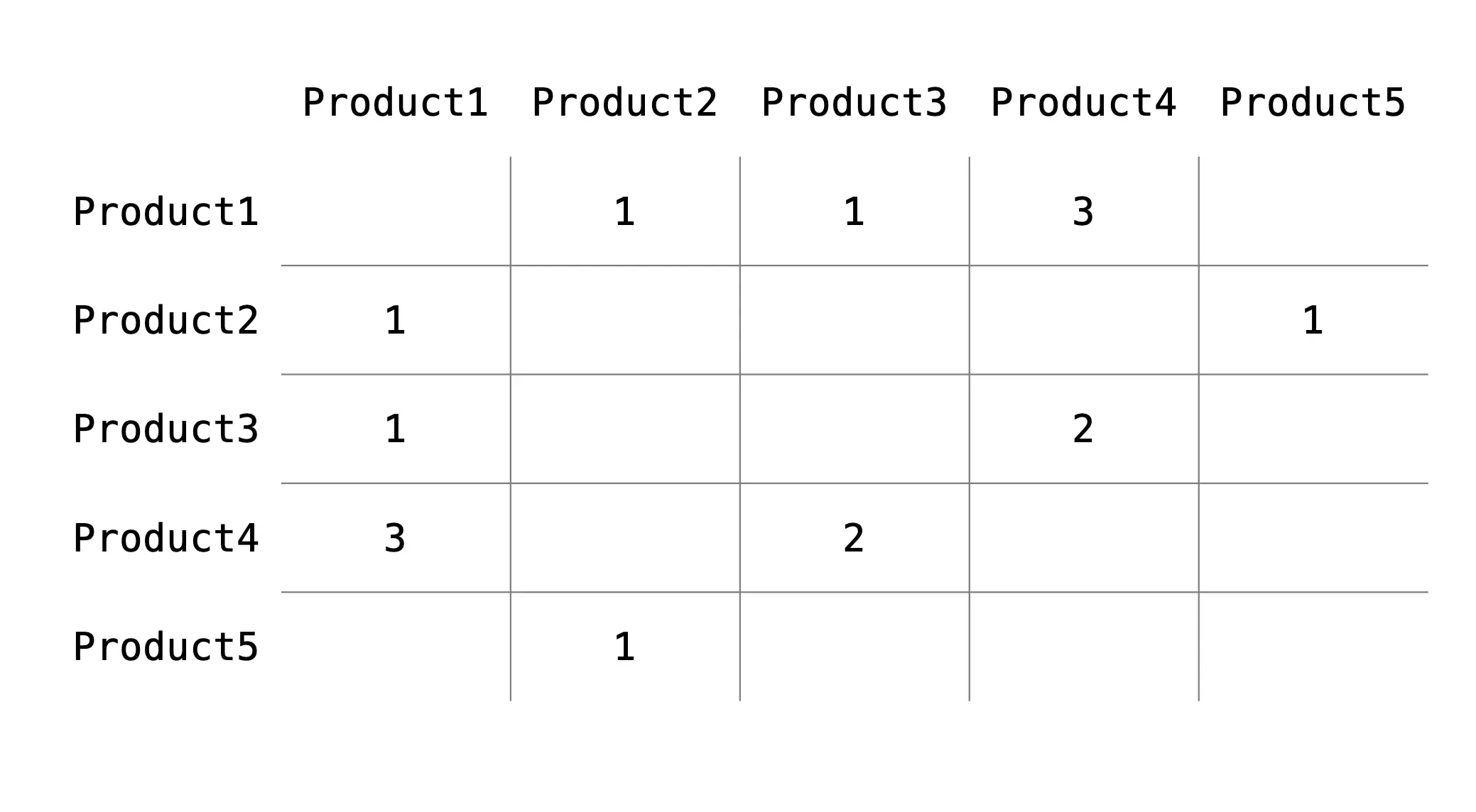
Figure 1c. Example weighted adjacency matrix

The adjacency matrix needs to be converted to a transition matrix, where the rows sum up to 1.0. Simply put, the transition matrix has the probability of each vertex transitioning to other vertices (thus each row summing to 1).

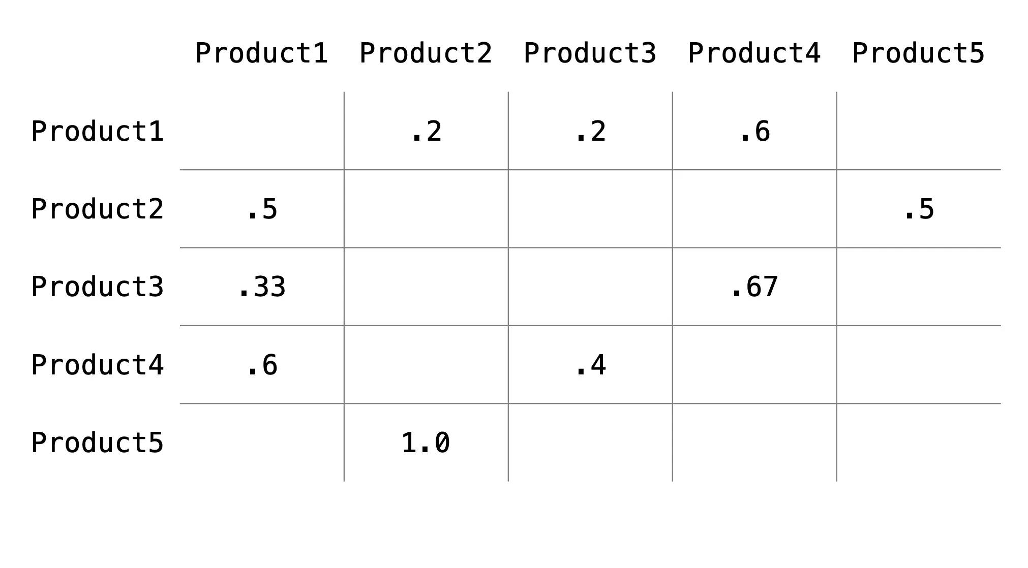
Figure 1d. Example transition matrix

My first attempt to calculate the transition matrix was using NumPy arrays as suggested here. It didn’t work due to memory constraints.

How can we make this more memory efficient?

Recall that the datasets have 99.99% sparsity. Of 420k electronics nodes, there are only 4 million edges. This means 420k**2 minus 4 million values are zero.

A regular NumPy array would initialize these zeros—which actually can be ignored—thus taking more memory than needed.

My next attempt involved sparse matrices (more about it here). In a nutshell, a sparse matrix doesn’t initialize those unnecessary zeros, saving memory. However, the matrix operations they support are not as extensive.

Converting the adjacency matrix to a transition matrix using sparse matrices worked. I’ll spare you the gory details.

With the transition matrix, I then converted it into dictionary form for the O(1) lookup goodness. Each key would be a node, and the value would be another dictionary of the adjacent nodes and the associated probability.

With this, creating random walks is now a lot simpler and much more efficient. The adjacent node can be identified by applying random.choice on the transition weights. This approach is orders of magnitude faster than traversing a networkx graph (Note: It is still traversing a graph).

Implementation 3: Node2Vec

(Implementation 3?! Where did 1 and 2 go—read the previous post.)

Soon after I went through the pain of building my own graph and sequences, I stumbled upon the github repository of Node2Vec (“n2v”) here. Note to self: Google harder before implementing something next time.

n2v was appealing—it seems to work right out of the box. You just need to provide the edges. It would then generate the graph and sequences, and learn node embeddings. Under the hood, it uses networkx and gensim.

Unfortunately, it was very memory intensive and slow, and could not run to completion, even on a 64gb instance.

Digging deeper, I found that its approach to generating sequences was traversing the graph. If you allowed networkx to use multiple threads, it would spawn multiple processes to create sequences and cache them temporarily in memory. In short, very memory hungry. Overall, this didn’t work for the datasets I had.

For the rest of the post, we’ll explore the training of product embeddings based on the sequences generated. To give you a better idea, these sequences are in the form of a NumPy array of objects (i.e., product IDs). The dimension is N x M, where N = number of unique products x 10, and Y = number of nodes per sequence.

Here’s how the sequences look like.

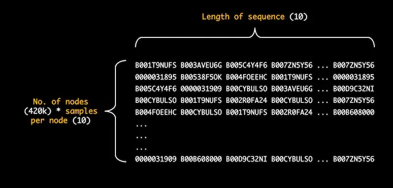
Figure 1e. Array of sequences for electronics dataset (420k unique products)

Implementation 4: gensim.word2vec

Gensim has an implementation of w2v that takes in a list of sequences and can be multi-threaded. It was very easy to use and the fastest to complete five epochs.

It performed significantly better than matrix factorization (in the previous post), achieving an AUC-ROC of 0.9082 (relative to ~0.8).

However, if you examine the precision recall curve below (Fig. 2), you’ll notice the sharp cliff at around threshold of 0.73—what’s causing this?

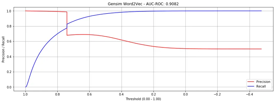
Figure 2. Precision recall curves for gensim.word2vec (all products)

The reason: “Unseen” products in our validation set without embeddings (i.e., they didn’t appear in the training set).

Gensim.w2v is unable to initialize / create embeddings for words that don’t exist in the training data. To get around this, for product-pairs in the validation set where either product doesn’t exist in the train set, we set the prediction score to the median similarity score. It is these unseen products that cause the sharp cliff.

If we only evaluate validation set product-pairs constituents that appeared in the training set, the performance is significantly improved to AUC-ROC = 0.9735 (Fig 3.). Also, no more cliffs.

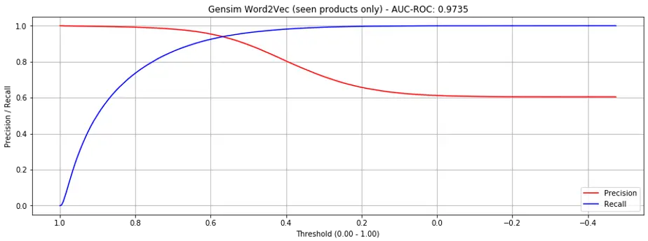
Figure 3. Precision recall curves for gensim.word2vec (seen products only)

Did I mention this runs in 2.58 minutes using 12 threads? This is the new baseline.

Great results in under 3 minutes—project complete, right?

Well, not really. The intent of this exercise is learning and trying new approaches. I also felt like I haven’t quite fully grokked w2v. Furthermore, with gensim, I couldn’t plot learning curves across batches and epochs.

Also, I’ve a few ideas on how to extend w2v for recsys and the vanilla gensim implementation doesn’t allow for extensions.

Therefore, let’s dive a bit deeper and implement it from scratch, in PyTorch.

Implementation 5: PyTorch word2vec

There are two main components to training a PyTorch model: The dataloader and the model. I’ll start with the more tedious dataloader.

The dataloader is largely similar to the previous implementation (for matrix factorization), with a few key differences. Firstly, instead of taking in product-pairs, it now takes in sequences.

Furthermore, there are two new features (i.e., subsampling of frequent words and negative sampling), both of which were proposed in the second w2v paper.

Subsampling of frequent words

In the paper, subsampling of frequent words (i.e., dropping out words that occur relatively frequently) was found to accelerate learning and significantly improve on learning vectors of rare words. This is fairly straightforward (an excellent explanation available here).

Negative sampling

Explaining negative subsampling is significantly more involved, so bear with me.

The original skip-gram had a (hierarchical) softmax layer at the end, where it outputs the probability of all vocabulary words being in the neighbourhood of the centre word.

If you had a vocabulary of 10k words (or products), that would be a softmax layer with 10k units. With an embedding dimension of 128, this means 1.28 million weights to update—that’s a lot of weights. This problem is more pronounced in recsys, as the “vocabulary” of products is in the millions.

Negative sampling only modifies a small proportion of weights. Specifically, the positive product-pair and a small sample of negative product-pairs. Based on the paper, five negative product-pairs is sufficient for most use cases.

If we have five negative product-pairs, this means we only need to update six output neurons (i.e., 1 positive product-pair, 5 negative product-pairs). Assuming 1 million products, that’s 0.0006% of the weights—very efficient!

(Note: You might have noticed that negative sampling was also adopted in the matrix factorization approach in the previous post, where five negative product-pairs were generated for each positive product-pair during training.)

How are these negative samples selected?

From the paper, they are selected using a unigram distribution, where more frequent words are more likely to be selected as negative samples. One unusual trick was to raise the word counts to the ¾ power, which they found to perform the best. This implementation does the same.

Skipgram model

For the model, the PyTorch w2v implementation is very straightforward and less than 20 lines of code, so I won’t go into explaining the details. Nonetheless, here’s some simplified code of how the skipgram model class looks like:

class SkipGram(nn.Module):
    def __init__(self, emb_size, emb_dim):
        self.center_embeddings = nn.Embedding(emb_size, emb_dim, sparse=True)
        self.context_embeddings = nn.Embedding(emb_size, emb_dim, sparse=True)

    def forward(self, center, context, neg_context):
        emb_center, emb_context, emb_neg_context = self.get_embeddings()

        # Get score for positive pairs
        score = torch.sum(emb_center * emb_context, dim=1)
        score = -F.logsigmoid(score)

        # Get score for negative pairs
        neg_score = torch.bmm(emb_neg_context, emb_center.unsqueeze(2)).squeeze()
        neg_score = -torch.sum(F.logsigmoid(-neg_score), dim=1)

        # Return combined score
        return torch.mean(score + neg_score)

How does it perform relative to matrix factorization?

Considering all products, the AUC-ROC achieved was 0.9554 (Fig. 4, significantly better than gensim). If only considering seen products, the AUC-ROC was 0.9855 (Fig. 5, slightly better than gensim).

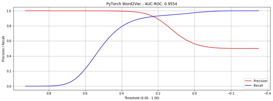
Figure 4. Precision recall curves for PyTorch word2vec (all products)

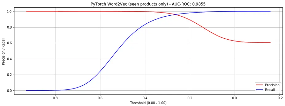
Figure 5. Precision recall curves for PyTorch word2vec (seen products only)

The results achieved here are also better than an Alibaba paper that adopted a similar approach, also on an Amazon electronics dataset. The paper reported an AUC-ROC of 0.9327.

When examining the learning curve (Fig. 6), it seems a single epoch is sufficient. What stands out is that each time the learning rate is reset (with each new epoch), the AUC-ROC doesn’t drop drastically as in matrix factorization.

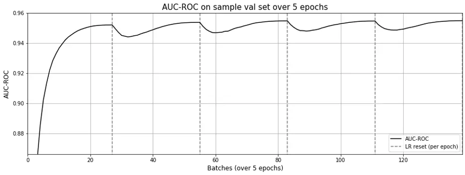
Figure 6. AUC-ROC across epochs for word2vec; a single epoch seems sufficient

Great result overall—it’s able to replicate gensim.word2vec and also does better.

Furthermore, it allows us to initialize embeddings for all products, even those not present in the train set. While those embeddings may be untrained, they can be updated with new data (without having to retrain from scratch).

One downside—it’s nowhere as efficient as the gensim implementation, taking 23.63 minutes. I blame my suboptimal implementation. (Suggestions on how to improve welcome!).

Implementation 6: PyTorch word2vec with side info

One reason why I built w2v from scratch is the intention of extending it by adding side information. For each product in a sequence, we have valuable side information such as brand, category, price, etc. (example below). Why not add this information when learning embeddings?

B001T9NUFS -> B003AVEU6G -> B007ZN5Y56 ... -> B007ZN5Y56
Television    Sound bar     Lamp              Standing Fan
Sony          Sony          Phillips          Dyson
500 – 600     200 – 300     50 – 75           300 - 400

Implementation-wise, instead of a single embedding per product, we now have multiple embeddings for product ID, brand, category, etc. We can then aggregate these embeddings into a single embedding.

This could potentially help with the cold-start problem; it was also proposed in the Alibaba paper where they used side information for brand, category level 1, and category level 2. By using a similar electronics dataset from Amazon, they reported AUC-ROC improvement (due to side information) from 0.9327 to 0.9575.

I implemented two versions. First, equal-weighted averaging (of embeddings) and second, learning the weightage for each embedding and applying a weighted average to aggregate into a single embedding.

Both didn’t work. AUC-ROC during training dropped to between 0.4 – 0.5 (Fig. 7).

Figure 7. AUC-ROC across epochs for word2vec with side information

After spending significant time ensuring the implementation was correct, I gave up. Trying it with no side information yielded the same results as implementation 5, albeit slower.

One possible reason for this non-result is the sparsity of the meta data. Out of 418,749 electronic products, we only had metadata for 162,023 (39%). Of these, brand was 51% empty.

Nonetheless, my assumption was that the weightage of the embeddings, especially the (less helpful) metadata embeddings, could be learned. Thus, their weight in the aggregate would be reduced (or minimized), and adding metadata should not hurt model performance. Clearly, this was not the case.

All in all, trying to apply w2v with side information didn’t work. ¯_(ツ)_/¯

Implementation 7: Sequences + Matrix Factorization

Why did the w2v approach do so much better than matrix factorization? Was it due to the skipgram model, or due to the training data format (i.e., sequences)?

To understand this better, I tried the previous matrix factorization with bias implementation (AUC-ROC = 0.7951) with the new sequences and dataloader.

Lo and behold, AUC-ROC shot up to 0.9320 (Fig. 8)!

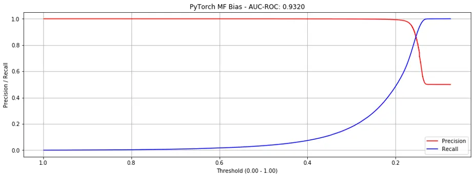
Figure 8. Precision recall curve for PyTorch MF-bias with sequences.

This suggests that the “graph-random-walk-sequences” approach works well.

One reason could be that in the original matrix factorization, we only learnt embeddings based on the product-pairs. But in the sequences, we used a window size of 5, thus we had 5 times more data to learn from, though products that are further apart in the sequences might be less strongly related.

Oddly though, the matrix factorization approach still exhibits the effect of “forgetting” as learning rate resets with each epoch (Fig 9.), though not as pronounced as Figure 3 in the previous post.

I wonder if this is due to using the same embeddings for both center and context.

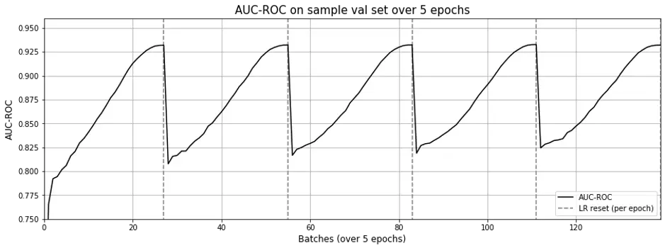
Figure 9. Learning curve for PyTorch MF-bias with sequences.

Another downside is that it takes about 3x the time, increasing from 23.63 minutes (w2v implementation) to 70.39 minutes (matrix factorization implementation).

Additional results on a bigger dataset (books)

In parallel, I also prepared a books dataset that has 2 million unique products making up 26.5 million product-pairs and applied the implementations on it.

Some notable results are as follows.

Matrix Factorization:

• Overall AUC-ROC: 0.4996 (not sure why it’s not able to learn)
• Time taken for 5 epochs: 1353.12 minutes

Gensim Word2vec

• Overall AUC-ROC: 0.9701
• Seen-products-only AUC-ROC: 0.9892
• Time taken for 5 epochs: 16.24 minutes

PyTorch Word2vec

• Overall AUC-ROC: 0.9775
• Time taken for 5 epochs: 122.66 minutes

PyTorch Matrix Factorization with Sequences

• Overall AUC-ROC: 0.7196
• Time taken for 5 epochs: 1393.08 minutes

Similarly, using sequences with matrix factorization helps significantly, though it doesn’t quite achieve the same stellar results as regular word2vec.

Further Extensions

In these two articles, we’ve examined 7 different item-to-item recsys implementations. And we haven’t even considered user information yet—the exploration space is huge!

If we have user data, we can build user embeddings in the same vector space (as product emdeddings). This can be done by training user embeddings based on the products that (i) users click on (positive), (ii) users are exposed to but don’t click on (negative), and (iii) purchase (strong positive).

This approach was adopted by Airbnb and seems promising. However, due to sparsity of user and product data (i.e., majority of users and accommodations have very few bookings), they aggregated users and accommodations into user and accommodation types—this ensures sufficient samples for each type.

Why stop at just user and product embeddings? From this exercise, we’ve seen how powerful embeddings can be with the right training data. In the StarSpace paper, Facebook has taken it to the extreme and propose to embed everything.

Recently, Uber Eats also shared about how they used Graph Neural Networks to learn embeddings for users and menu items, where a node’s embedding is based on it neighbours. More here.

Key Takeaways

Using w2v to generate product embeddings is a very strong baseline and easily beats basic matrix factorization approaches.

If you have the sequences ready, you can just use gensim’s implementation. If you want to extend on w2v and need your own implementation, developing it is not difficult.

It was great that the PyTorch w2v implementation did better than gensim’s, and had better results than the Alibaba paper. Unfortunately, I was unable to replicate the improvements from using side information. Perhaps I need to rerun the experiments on a dataset where the metadata is less sparse to confirm.

Lastly, training data in the form of sequences are epic—matrix factorization with sequences is far better than just matrix factorization with product-pairs. Sequences can be built via multiple novel approaches—in this post, I built a product graph and then performed random walks to generate those sequences.

Conclusion

This has been a fun exercise to apply my interest in sequences to an area of machine learning where they are less commonly seen (i.e., recsys).

I hope the learnings and code shared here will be useful for others who are developing their own recsys implementations, be it for fun or at work.

P.S. Looking for the code for this? Available on github: recsys-nlp-graph

References

Mikolov, T., Sutskever, I., Chen, K., Corrado, G. S., & Dean, J. (2013). Distributed representations of words and phrases and their compositionality. In Advances in neural information processing systems (pp. 3111-3119).

Mikolov, T., Chen, K., Corrado, G., & Dean, J. (2013). Efficient estimation of word representations in vector space. arXiv preprint arXiv:1301.3781.

Perozzi, B., Al-Rfou, R., & Skiena, S. (2014, August). Deepwalk: Online learning of social representations. In Proceedings of the 20th ACM SIGKDD international conference on Knowledge discovery and data mining (pp. 701-710). ACM.

Grover, A., & Leskovec, J. (2016, August). node2vec: Scalable feature learning for networks. In Proceedings of the 22nd ACM SIGKDD international conference on Knowledge discovery and data mining (pp. 855-864). ACM.

Wang, J., Huang, P., Zhao, H., Zhang, Z., Zhao, B., & Lee, D. L. (2018, July). Billion-scale commodity embedding for e-commerce recommendation in alibaba. In Proceedings of the 24th ACM SIGKDD International Conference on Knowledge Discovery & Data Mining (pp. 839-848). ACM.

Grbovic, M., & Cheng, H. (2018, July). Real-time personalization using embeddings for search ranking at airbnb. In Proceedings of the 24th ACM SIGKDD International Conference on Knowledge Discovery & Data Mining (pp. 311-320). ACM.

Wu, L. Y., Fisch, A., Chopra, S., Adams, K., Bordes, A., & Weston, J. (2018, April). Starspace: Embed all the things!. In Thirty-Second AAAI Conference on Artificial Intelligence.

Food Discovery with Uber Eats: Using Graph Learning to Power Recommendations, https://eng.uber.com/uber-eats-graph-learning/, retrieved 10 Jan 2020

Thanks to Basil Han for suggesting bug fixes.

If you found this useful, please cite this write-up as:

Yan, Ziyou. (Jan 2020). Beating the Baseline Recommender with Graph & NLP in Pytorch. eugeneyan.com. https://eugeneyan.com/writing/recommender-systems-graph-and-nlp-pytorch/.

or

@article{yan2020graph,
  title   = {Beating the Baseline Recommender with Graph & NLP in Pytorch},
  author  = {Yan, Ziyou},
  journal = {eugeneyan.com},
  year    = {2020},
  month   = {Jan},
  url     = {https://eugeneyan.com/writing/recommender-systems-graph-and-nlp-pytorch/}
}