P.S. Looking for the code for this? Available on github: recsys-nlp-graph

Recommender systems (“recsys”) are a fairly old topic that started back in the 1990s. The key idea—we can use opinions and behaviours of users to suggest and personalize relevant and interesting content for them.

Adding yet another post on the standard item-user collaborative filtering wouldn’t contribute much to the hundreds, if not thousands, of posts available.

Thankfully, this is not one of those.

Overview

A web search on recommender systems surfaces articles on “collaborative filtering”, “content-based”, “user-item matrix”, etc.

Since then, there has been much progress applying newer techniques for recsys. Unfortunately, easily readable articles or blogs on them are few and far between.

Thus, in this pair of articles, I’ll be sharing about seven different implementations of recsys.

The articles cover the end-to-end, from data acquisition and preparation, and (classic) matrix factorization. It also includes applying techniques from graphs and natural language processing. A result comparison of the different approaches on real-world data will also be discussed (I hope you love learning curves.)

Data Acquisition

We can’t build a recsys without data (well, we can’t build most machine learning systems without data).

Thankfully, Professor Julian McAuley, Associate Professor at UC San Diego has a great collection of data sets (e.g., product reviews, meta data, social networks). For this post, we’ll be using the Amazon dataset (May 1996 – July 2014), specifically, the electronics and books datasets.

Parsing json

All of the datasets are in json format and require parsing into a format that’s easier to work with (e.g., tabular). Some of these datasets can be pretty large, with the largest having 142.8 million rows and requiring 20gb on disk.

Here’s an example of how a json entry for a single product looks like (what we’re interested in is the related field).

{ 
"asin": "0000031852",
"title": "Girls Ballet Tutu Zebra Hot Pink",
"price": 3.17,
"imUrl": "http://ecx.images-amazon.com/images/I/51fAmVkTbyL._SY300_.jpg",
"related”:
    { "also_bought":[
		  	"B00JHONN1S",
		  	"B002BZX8Z6",
		  	"B00D2K1M3O", 
		  	...
		  	"B007R2RM8W"
                    ],
      "also_viewed":[ 
		  	"B002BZX8Z6",
		  	"B00JHONN1S",
		  	"B008F0SU0Y",
		  	...
		  	"B00BFXLZ8M"
                     ],
      "bought_together":[ 
		  	"B002BZX8Z6"
                     ]
    },
"salesRank":
    { 
      "Toys & Games":211836
    },
"brand": "Coxlures",
"categories":[ 
	    [ "Sports & Outdoors",
	      "Other Sports",
	      "Dance"
	    ]
    ]
}

Needless to say, we’re not going to be able to load this fully into ram on a regular laptop with 16gb ram (which I used for this exercise).

To parse the json to csv, I iterated through the json file row by row, converted the json into comma-delimited format, and wrote it out to CSV. (Note: This requires that we know the full keys of the json beforehand).

At the end, we have product metadata in nice tabular format. This includes columns for title and description, brand, categories, price, and related products.

Getting product relationships

To get the product relationships, we need the data in the “related” field. This contains relationships on “also bought”, “also viewed”, “bought together”, etc.

Extracting this requires a bit of extra work as it is contained in a dictionary of lists. Did I mention that it’s also in string format?

To get the relationships, we take the following steps:

• Evaluate the string and convert to dictionary format
• Get the associated product IDs for each relationship
• Explode it so each product-pair is a single row with a single relationship

In the end, what we have is a skinny three column table, with columns for product 1, product 2, and relationships (i.e., also bought, also viewed, bought together). At this point, each product pair can have multiple relationships between them.

Here’s a sample:

product1   | product2   | relationship
--------------------------------------
B001T9NUFS | B003AVEU6G | also_viewed
0000031895 | B002R0FA24 | also_viewed
B007ZN5Y56 | B005C4Y4F6 | also_viewed
0000031909 | B00538F5OK | also_bought
B00CYBULSO | B00B608000 | also_bought
B004FOEEHC | B00D9C32NI | bought_together

Converting relationships into a single score

Now that we have product-pairs and their relationships, we’ll need to convert them into some kind of single score/weight.

For this exercise, I’ll simplify and assume the relationships are bidirectional (i.e., symmetric in direction). (Note: Product-pair relationships can be asymmetric; people who buy phones would also buy a phone case, but not vice versa).

How do we convert those relationship types into numeric scores?

One simple way is to assign 1.0 if a product-pair have any/multiple relationships, and 0.0 otherwise.

However, this would ignore the various relationship types—should a product pair with an “also bought” relationship have the same score as one that has an “also viewed” relationship?

To address this, weights were assigned based on relationships (bought together = 1.2, also bought = 1.0, also viewed = 0.5) and summed across all unique product pairs. This results in a single numeric score for each product pair (sample below).

product1   | product2   | weight
--------------------------------
B001T9NUFS | B003AVEU6G | 0.5
0000031895 | B002R0FA24 | 0.5
B007ZN5Y56 | B005C4Y4F6 | 0.5
0000031909 | B00538F5OK | 1.0
B00CYBULSO | B00B608000 | 1.0
B004FOEEHC | B00D9C32NI | 1.2

For the electronics dataset, there’re 418,749 unique products and 4,005,262 product-pairs (sparsity = 4 million / 420k ** 2 = 0.9999). For books, we have 1,948,370 unique products, and 26,595,848 product pairs (sparsity=0.9999).

Yeap, recommendation data is very sparse.

Train-validation split

The data sets were randomly split into 2/3 train and 1/3 validation. This can be done with sklearn.train_val_split or random indices. Easy-peasy.

Done, amirite?

Unfortunately, not.

You might have noticed that our dataset of product-pairs consists only of positive cases. Thus, for our validation set (and the training set during training time), we need to create negative samples.

Creating negative samples in an efficient manner is not so straightforward.

Assuming we have 1 million positive product-pairs, to create a validation set with 50:50 positive-negative pairs would mean 1 million negative samples.

If we randomly (and naïvely) sample from our product pool to create these negative samples, it would mean random sampling 2 million times. Calling random these many times takes very long—believe me, I (naïvely) tried it.

To get around this, I applied this hack:

• Put the set of products in an array
• Shuffle the array

For each iteration, take a slice of the array at the iteration x 2

• If iteration = 0, product-pair = array[0: 0+2]
• If iteration = 1, product-pair = array[2:, 2+2]
• If iteration = 10, product-pair = array[20: 20+2]
• Once the array is exhausted, (re)shuffle and repeat

This greatly reduced the amount of random operations required and was about 100x faster than the naïve approach.

Collaborating filtering (how it is commonly known)

Collaborative filtering uses information on user behaviours, activities, or preferences to predict what other users will like based on item or user similarity. In contrast, content filtering is based solely on item metadata (i.e., brand, price, category, etc.).

Most collaborative filtering articles are on user-item collaborative filtering (more specifically, matrix factorization). And there’s always an (obligatory) user-item matrix (Fig. 1).

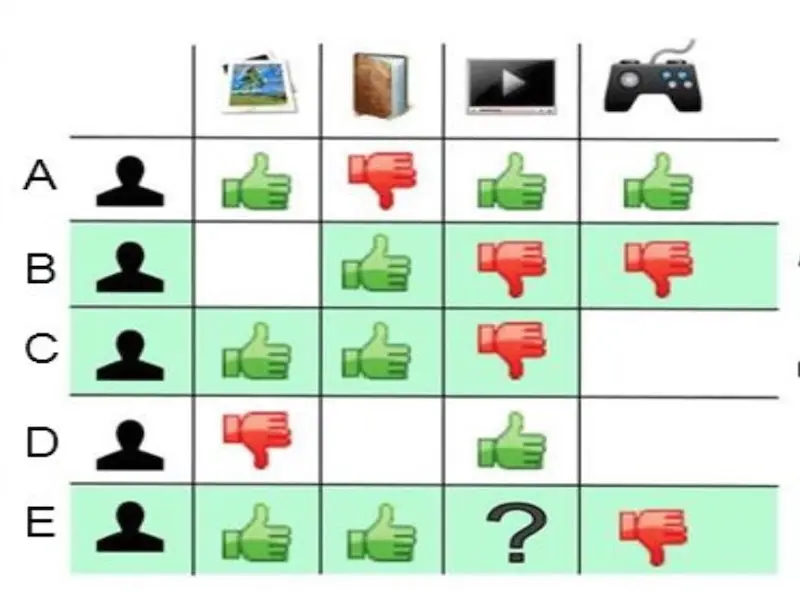
Figure 1. Cliché representation of collaborative filtering

However, if we don’t have user data (like in this case), can this still work?

Why not?

Instead of a user-item matrix, we have an item-item matrix. We then learn latent factors for each item and determine how strongly they’re related to other items.

One way to do this is to load the entire item-item matrix (in memory) and apply something like Python’s surprise or SparkML’s Alternating Least Squares.

However, this can be very resource intensive if you have to load the entire dataset into memory or apply some distributed learning approach.

Our datasets are very sparse (99.99% empty). Can we make use of the sparsity to make it more resource efficient? (Hint: Yes, we can.)

Implementation 1: Matrix Factorization (iteratively pair by pair)

One way to reduce the memory footprint is to perform matrix factorization product-pair by product-pair, without fitting it all into memory. Let’s discuss how to implement this in PyTorch.

First, we load the product-pairs (just the pairs, not the entire matrix) into an array. To iterate through all samples, we just need to iterate through the array.

Next, we need to create negative product-pair samples. Here’s the approach taken to generate negative samples:

• For each product pair (e.g., 001-002), we take the product on the left (i.e., 001) and pair it with n (e.g., five) negative product samples to form negative product-pairs
• The negative samples are based on the set of products available, with the probability of each product being sampled proportional to their frequency of occurrence in the training set

Thus, each (positive) product-pair (i.e., 001-002) will also have five related negative product-pairs during training.

Continous labels

For each product-pair, we have numeric scores based on some weightage (bought together = 1.2, also bought = 1.0, also viewed = 0.5). Let’s first train on these continuous labels. This is similar to working with explicit ratings.

Binary labels

To do it in the binary case (such as with implicit feedback), actual scores greater than 0 are converted to 1. Then, a final sigmoid layer is added to convert the score to between 0 – 1. Also, we use a loss function like binary cross entropy (BCE).

Regularization

Regularization—no doubt it’s key in machine learning. How can we apply it?

One approach is adding L2 regularization to ensure embeddings weights don’t grow too large. We do this by by adding a cost of sum(embedding.weights**2) * C (regularization param) to the total loss.

At a high level, for each pair:

• Get the embedding for each product
• Multiply embeddings and sum the resulting vector (this is the prediction)
• Reduce the difference between predicted score and actual score (via gradient descent and a loss function like mean squared error or BCE)

Here’s some pseudo-code on how iterative matrix factorization would work:

for product_pair, label in train_set:
    # Get embedding for each product
    product1_emb = embedding(product1)
    product2_emb = embedding(product2)

    # Predict product-pair score (interaction term and sum)
    prediction = sig(sum(product1_emb * product2_emb, dim=1))
    l2_reg = lambda * sum(embedding.weight ** 2) 

    # Minimize loss
    loss = BinaryCrossEntropyLoss(prediction, label)
    loss += l2_reg

    loss.backward()
    optimizer.step()

Training Schedule

For the training schedule, we run it over 5 epochs with cosine annealing. For each epoch, learning rate starts high (0.01) and drops rapidly to a minimum value near zero, before being reset for to the next epoch (Fig. 2).

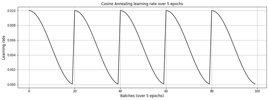
Figure 2. Cosine Annealing learning rate schedule

Results

For the smaller electronics dataset (420k unique products with 4 million pairs), it took 45 minutes for 5 epochs—doesn’t seem too bad.

Training on binary labels (1 vs. 0), we get a ROC-AUC of 0.8083. Not bad considering that random choice leads to ROC-AUC of 0.5.

From the learning curve (Fig. 3) below, you’ll see that one epoch is sufficient to achieve close to optimal ROC-AUC. Interestingly, each time the learning rate is reset, the model seems to need to “relearn” the embeddings from scratch (AUC-ROC drops to near 0.5).

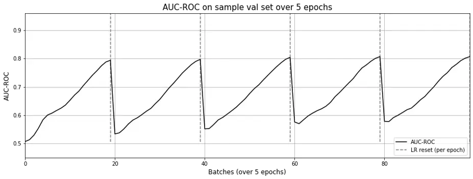
Figure 3. AUC-ROC across epochs for matrix factorization; Each time learning rate is reset, the model seems to ”forget”, causing AUC-ROC to revert to ~0.5. Also, a single epoch seems sufficient.

However, if we look at the precision-recall curves below (Fig. 4), you see that at around 0.5 we hit the “cliff of death”. If we estimate the threshold slightly too low, precision drops from close to 1.0 to 0.5; slightly too high and recall is poor.

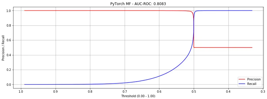
Figure 4. Precision recall curves for Matrix Factorization (binary labels).

Using the continuous labels, performance seems significantly better (AUC-ROC = 0.9225) but we see the same cliff of death (Fig. 5). Nonetheless, this does suggest that explicit (i.e., scale) ratings can perform better than implicit ratings.

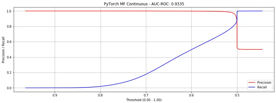
Figure 5. Precision recall curves for Matrix Factorization (continuous labels).

This baseline model only captures relationships between each product. But what if a product is generally popular or unpopular?

We can add biases. Implementation wise, it’s a single number for each product.

Implementation 2: Matrix Factorization with Bias

If we just observe the AUC-ROC metric, adding bias doesn’t seem to help, where AUC-ROC decreases from 0.8083 to 0.7951 on binary labels, and from 0.9335 to 0.8319 on continuous labels.

However, if we examine the precision-recall curves, adding bias reduces the steepness of the curves where they intersect, making it more production-friendly (i.e., putting it into production). Here are the curves for both binary (Fig. 6) and continuous labels (Fig. 7).

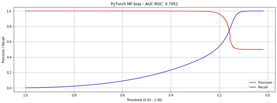
Figure 6. Precision recall curves for Matrix Factorization + bias (binary labels).

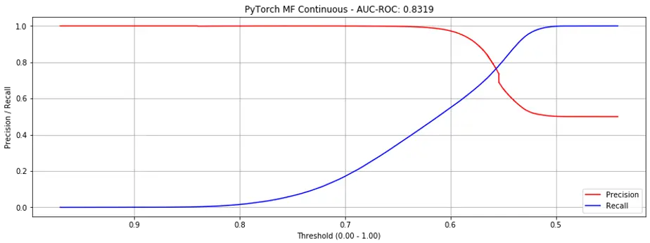
Figure 7. Precision recall curves for Matrix Factorization + bias (continuous labels).

It may seem alarming that AUC-ROC on continuous labels drops sharply (0.9335 to 0.8319), but it shouldn’t be—it’s an artefact of how AUC-ROC is measured.

In the ROC curve for the continuous labels without bias (Fig. 8a), false positives only start to occur after about 0.75 of true positives are identified. Beyond the threshold of 0.5, all false positives are introduced (i.e., precision curve cliff of death in Fig. 5). The ROC curve and AUC-ROC metric doesn’t make this very observable and the AUC-ROC appears significantly better (but it really isn’t).

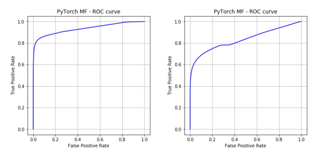
Figure 8a (left) and 8b (right). ROC curves with and without bias.

On the larger books dataset, it took about 22 hours for 5 epochs—this approach seems to scale more than linearly based on the number of product-pairs (i.e., scales badly). Unfortunately, the AUC-ROC stays around 0.5 during training.

Key takeaways

The (iterative) matrix factorization approach seems to do okay for a baseline, achieving decent AUC-ROC of ~0.8.

While the baseline approach (without bias) does well, it suffers from sharp cliffs on the precision curve. Adding bias improves on this significantly.

More importantly, we learnt that one shouldn’t just look at numeric metrics to understand how a machine learning model is doing. Plotting the curves can be very useful to better understand how your model performs, especially if it’s classification-based and you need to arbitrarily set some threshold.

What’s next?

Wait, isn’t this still matrix factorization, albeit in an iterative, less memory-intensive form? Where’s the graph and NLP approaches? You tricked me!

Yes, the current post only covers the baseline, albeit in an updated form.

Before trying any new-fangled techniques, we have to first establish a baseline, which is what this post does.

In the next post, we’ll apply graph and NLP techniques to the problem of recommender systems.

P.S. Looking for the code for this? Available on github: recsys-nlp-graph

References

McAuley, J., Targett, C., Shi, Q., & Van Den Hengel, A. (2015, August). Image-based recommendations on styles and substitutes. In Proceedings of the 38th International ACM SIGIR Conference on Research and Development in Information Retrieval (pp. 43-52). ACM.

If you found this useful, please cite this write-up as:

Yan, Ziyou. (Jan 2020). Building a Strong Baseline Recommender in PyTorch, on a Laptop. eugeneyan.com. https://eugeneyan.com/writing/recommender-systems-baseline-pytorch/.

or

@article{yan2020matrix,
  title   = {Building a Strong Baseline Recommender in PyTorch, on a Laptop},
  author  = {Yan, Ziyou},
  journal = {eugeneyan.com},
  year    = {2020},
  month   = {Jan},
  url     = {https://eugeneyan.com/writing/recommender-systems-baseline-pytorch/}
}