In a previous post, we discussed diffusers and the process of diffusion, where we gradually add noise to data and then learn how to remove the noise. If you’re familiar with autoencoders, this may seem similar to the denoising variant. Let’s take a look at how they compare. But first, a brief overview of autoencoders.

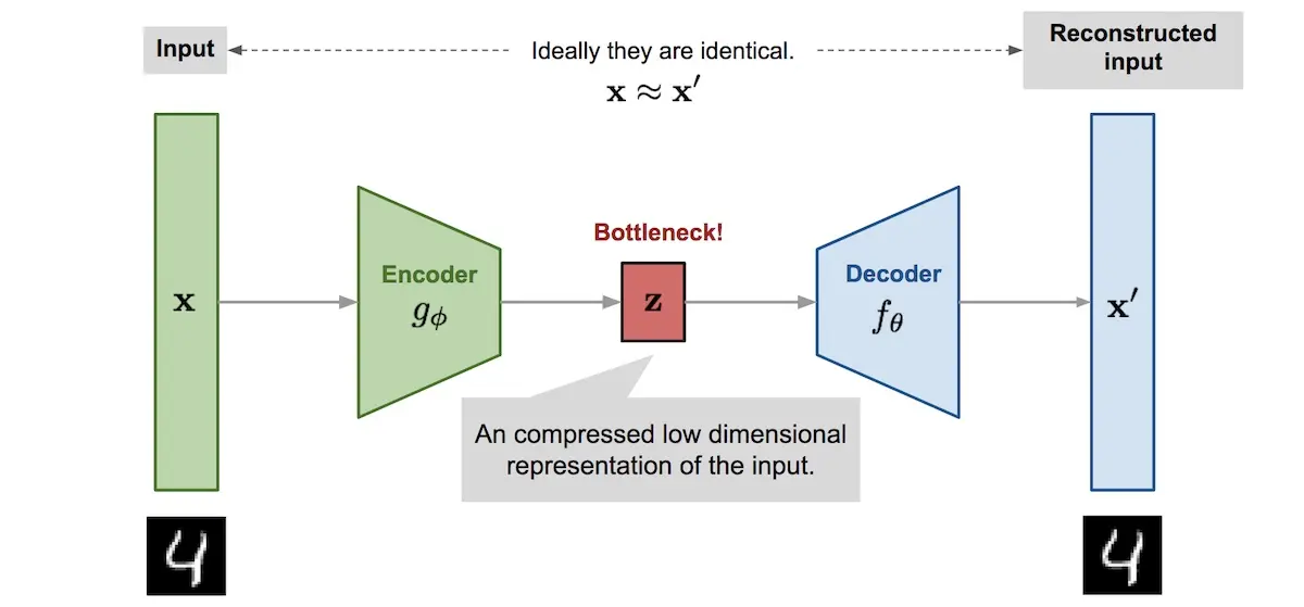
Autoencoders are neural networks trained to predict their input: Given an input, reproduce it as the output. This is meaningless unless we constrain the network in some way. The typical constraint is a bottleneck layer that limits the amount of information that can pass through. For example, a hidden layer—between the encoder and decoder—that has a much lower dimension relative to the input. With this constraint, the network learns which information to pass through the bottleneck so that it can reproduce the output.

Autoencoder architecture with the bottleneck layer (source)

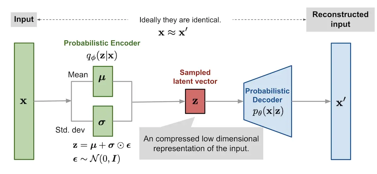
A variation of the autoencoder is the variational autoencoder. Instead of mapping the input to a fixed vector (via the bottleneck layer), it maps it to a distribution. In the case of a Gaussian distribution, the mean (\(\mu\)) and variance (\(\sigma\)) of the distribution can be learned via the reparameterization trick. (Also see the informal and formal explanations for the reparameterization trick).

Variational autoencoder with multivariate Gaussian assumption (source)

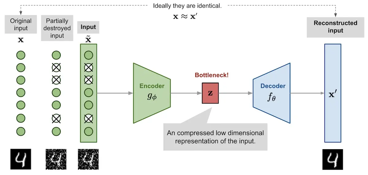
Another variant is the denoising autoencoder, where the input is partially corrupted by adding noise or masking values randomly. The model is then trained to return the original input without the noise. To denoise the noisy input, the autoencoder has to learn the relationship between input values, such as image pixels, to infer the missing pieces. As a result, the autoencoder is more robust and can generalize better. (Adding noise was motivated by humans being able to recognize an object even if it’s partially occluded.)

Denoising autoencoder with the corrupted input (source)

Put another way, autoencoders learn to map the input data in a lower-dimensional manifold of the naturally occurring data (more on manifold learning). In the case of denoising autoencoders, by mapping the noisy input to the manifold region and then decoding it, they are able to reconstruct the input without the noise.

I think autoencoders and diffusers are similar in some ways. Both have a similar learning paradigm: Given some data as input, reproduce it as output (and learn the data manifold in the process). In addition, both have similar architectures that use bottleneck layers, where we can view U-Nets as autoencoders with residual connections to improve gradient flow. Also, in the case of the denoising autoencoder, the approach of corrupting the input and learning to denoise it. Taken together, both models are similar in learning a lower-dimensional manifold of the data.

The key difference lies in diffusion models conditioning on the timestep (\(t\)) as input. This allows a single diffusion model—and a single set of parameters—to handle different noise levels. As a result, a single diffusion model can generate (blurry) images from noise at high \(t\) and then sharpen them at lower \(t\). Current diffusion models also condition on text, such as image captions, letting them generate images based on text prompts.

• • •

That’s all in this brief overview of autoencoders and how they compare with diffusion models. Did I miss anything? Please reach out!

If you found this useful, please cite this write-up as:

Yan, Ziyou. (Dec 2022). Autoencoders and Diffusers: A Brief Comparison. eugeneyan.com. https://eugeneyan.com/writing/autoencoders-vs-diffusers/.

or

@article{yan2022autoencoder,
  title   = {Autoencoders and Diffusers: A Brief Comparison},
  author  = {Yan, Ziyou},
  journal = {eugeneyan.com},
  year    = {2022},
  month   = {Dec},
  url     = {https://eugeneyan.com/writing/autoencoders-vs-diffusers/}
}