Text-to-image has advanced at a breathless pace in 2021 - 2022, starting with DALL·E, then DALL·E 2, Imagen, and now Stable Diffusion. I dug into a couple of papers to learn more about the space and organized my understanding into a few key concepts:

• Diffusion: Gradually add noise to data and then learn to generate data from noise
• Text conditioning: Generating images given (i.e., conditioned on) a text prompt
• Classifier guidance: Using classifier gradients to text-increase image alignment
• Latent space: Applying diffusion on image embeddings instead of image pixels

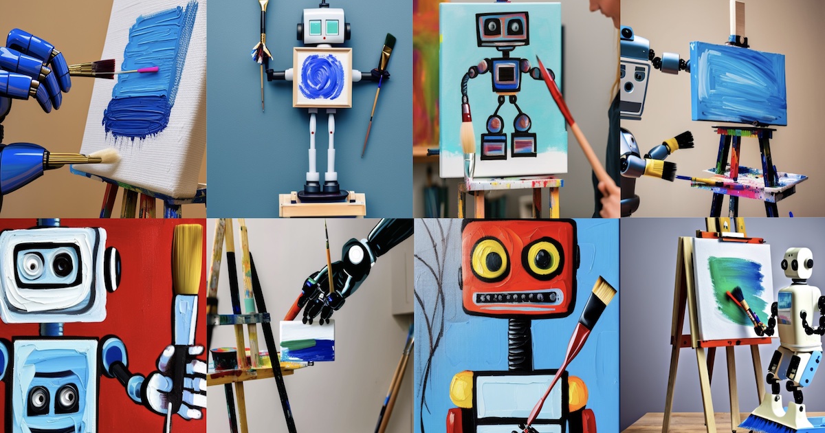
OG image prompt: "a robot holding a paint brush painting on an art stand"

Diffusion: From data to noise and back

Let’s start with the earliest diffusion paper I know, cryptically titled “Deep Unsupervised Learning using Nonequilibrium Thermodynamics, by Sohl-Dickstein in 2015. In it, the authors explained that the idea of diffusion was inspired by non-equilibrium statistical physics (perhaps the particle physics concept with the same name?)

The key idea is to gradually destroy structure in a data distribution (e.g., image) via a forward diffusion process, and then learn a reverse diffusion process (via a model) to restore the structure in the data. And once we have a trained model, we can generate images by starting from pure noise and applying reverse diffusion (aka sampling).

To implement forward diffusion, they apply a Markov chain that progressively adds Gaussian noise to the data until the signal is destroyed (i.e., complete noise).

For reverse diffusion, they train a diffusion probabilistic model (DPM) to transform noised images to less noisy images. Reverse diffusion is done via many small denoising steps, instead of a single large step from pure noise to clean image—the intuition is that taking many small steps is more tractable than a single large step.

They shared an example of diffusion on 2d Swiss roll data. Forward diffusion (top in blue, left to right) gradually adds Gaussian noise until the data is pure noise. Reverse diffusion (middle in red, right to left) gradually denoises the data to get back the 2d swiss roll.

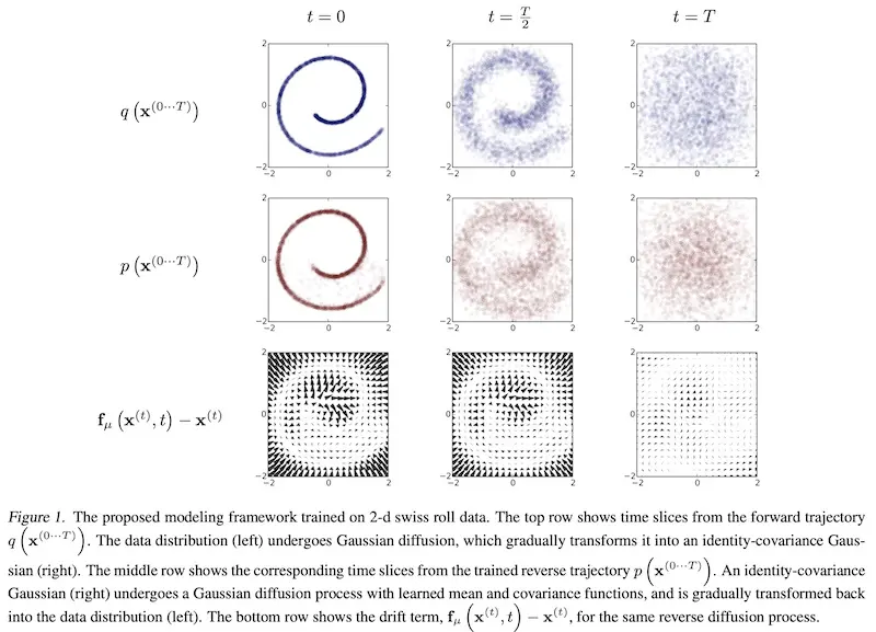
Forward (blue) and backward (red) diffusion process (source)

Denoising Diffusion Probabilistic Models (DDPM; 2020) shares a gentler explanation of the diffusion process: Forward diffusion (\(q\)) is a predefined process that gradually adds Gaussian noise to the image until it’s pure noise. Reverse diffusion (\(p\)) is a learned process that gradually denoises an image starting from pure noise until we get an actual image.

Forward (q) and backward (p) diffusion process (source)

If we knew the conditional distribution of \(p(x_{t-1}\vert x_{t})\), we could just run the forward diffusion process in reverse: Sample random Gaussian noise (\(x_{t}\)) and denoise it to get a sample image from the real distribution.

Unfortunately, we don’t know \(p(x_{t-1}\vert x_{t})\) as it’s intractable—it requires knowing the distribution of all possible images to compute the conditional probability. Thus, we train a model (i.e., neural network) to learn the conditional probability distribution \(p_{\theta}(x_{t-1}\vert x_{t})\), where \(\theta\) are the model parameters.

Given that the forward diffusion process is Gaussian (since the added noise is Gaussian), perhaps we can assume the reverse process to be Gaussian too. If so, reverse diffusion can be represented via mean (\(\mu_{\theta}\)) and variance (\(\Sigma_{\theta}\)) and be parameterized as:

In layman’s terms, the probability of the less noisy image (\(x_{t-1}\)) given a noisier image (\(x_{t}\)) from the previous timestep (\(t\)) is drawn from a Gaussian distribution (\(\mathcal{N}\)) where the mean is the mean of \(x_{t}\) at timestep \(t\) and the variance is the variance of \(x_{t}\) at timestep \(t\). Thus, the neural network needs to learn the mean (\(\mu_{\theta}\)) and variance (\(\Sigma_{\theta}\)). That said, in DDPM, the variance is predefined and the network only has to learn the mean.

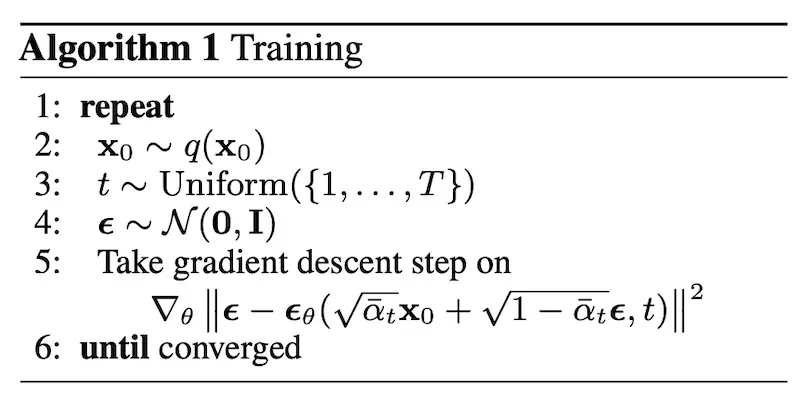
Training algorithm for DDPM (source)

Here’s a step-by-step of the training algorithm:

• Line 1: Start while loop
• Line 2: Sample a random clean image (\(x_{0}\)) from the set of images
• Line 3: Sample a noise level (\(t\)) uniformly from 1 to max \(T\)
• Line 4: Sample some noise (\(\epsilon\)) from a Gaussian and corrupt image with the noise
• Line 5: Train the neural network to predict the noise based on the corrupted image
• Line 6: End while loop when model converges

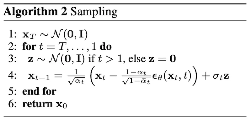
Sampling algorithm for DDPM (source)

When we have a trained model, here’s how to generate new images starting from noise:

• Line 1: Get a sample noise image (\(x_{T}\)) from a Gaussian distribution
• Line 2: Iterate from timestep \(T\) to timestep 1
• Line 3: Sample additional Gaussian noise (\(z\) if timestep > 1 else zero, because we just return the clean image at timestep 1)
• Line 4: Get the slightly denoised image (\(x_{t-1}\)) by subtracting the noise (\(\epsilon_{\theta}(x_{t}, t)\)) from the noisy image (\(x_{t}\)), and then adding back some noise (\(z\))
• Line 5: End iteration
• Line 6: Return clean image from timestep 1

Notice the model predicts all the noise from a noisy image (\(\epsilon_{\theta}(x_{t}, t)\)). However, we only subtract a fraction of it, weighted by \(\frac{1-\sigma_{t}}{\sqrt{}1-\bar{\sigma_{t}}}\), and then add back noise (\(z\)) weighted by \(\sigma_{t}\).

I was curious about these noise removal and addition weights and coded up a DDPM to tinker with it. To my surprise, the noise removal weights are as low as 0.01 to 0.02 while the noise addition weights go as high as 0.14. Remember the intuition that estimating small amounts of noise for multiple timesteps is more tractable than estimating all noise via a single timestep? This is how it’s implemented in the algorithm and code.

t = 799 - Latent weight: 1.010, Removed noise weight: 0.020, Added noise weight: 0.141
t = 640 - Latent weight: 1.008, Removed noise weight: 0.016, Added noise weight: 0.127
t = 480 - Latent weight: 1.006, Removed noise weight: 0.012, Added noise weight: 0.110
t = 320 - Latent weight: 1.004, Removed noise weight: 0.009, Added noise weight: 0.090
t = 160 - Latent weight: 1.002, Removed noise weight: 0.008, Added noise weight: 0.064
t = 0   - Latent weight: 1.000, Removed noise weight: 0.010, Added noise weight: 0.000

Weights for the latent, noise removal, and noise addition at t = 799, 640, 480, 320, 160, 0 (source)

Via experimenting with the DDPM, I learned that more timesteps had a positive impact on sample quality though it also required more epochs and a large timestep embedding. Larger dimensions for the timestep embedding also improved loss and sample quality. On the other hand, more epochs, different loss functions, and batch size didn’t help. (Want to understand diffusion better? Clone this GitHub repo and play with the code!)

So far, these models are only capable of basic diffusion (i.e., generating images from noise, limited by the dataset they’re trained on). They are unable to generate images from text prompts (unlike DALL·E and Stable Diffusion)—to do this, we need text conditioning.

(Aside: I thought the approach of corrupting input with noise and learning to remove the noise was similar to denoising autoencoders and wrote a brief comparison.)

Text conditioning: Influencing image output via text

To understand text conditioning, I think it helps to start with Contrastive Language-Image Pre-training (CLIP; 2021). It embeds text and image in the same space via a projection layer. Thus, it can efficiently learn visual concepts, in the form of text, via natural language supervision and perform zero-shot classification.

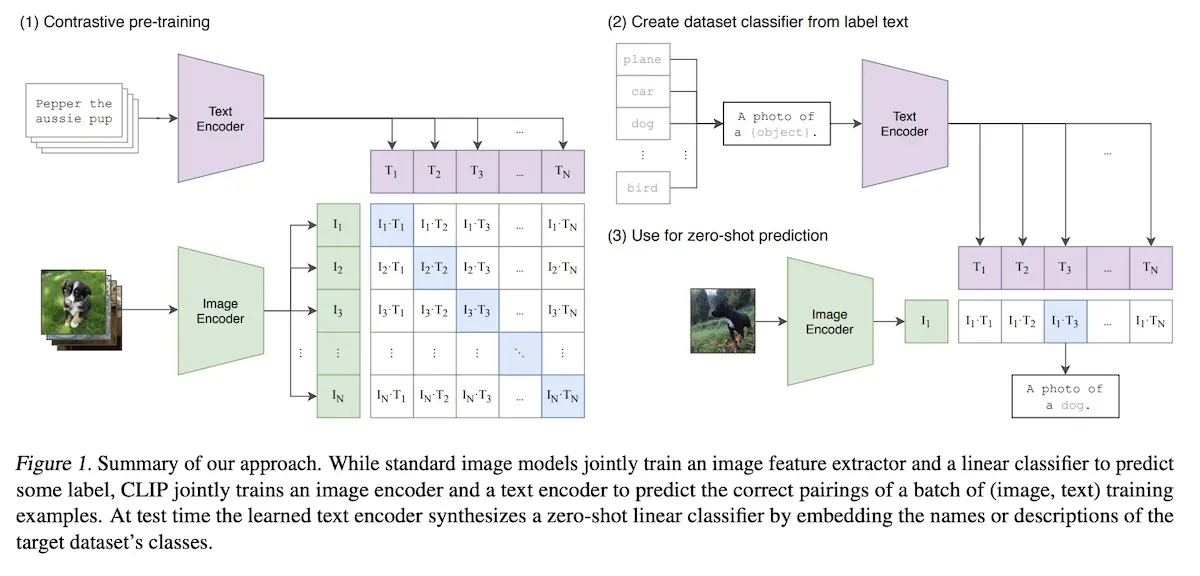
CLIP pre-training and zero-shot classification (source)

In the pre-training stage, the image and text encoders are trained to predict which images are paired with which texts in a dataset of 400M image-caption pairs. CLIP is trained to maximize the cosine similarity of the image and text embeddings of image-caption pairs via a multi-modal embedding space.

This is implemented via a linear projection to map each encoder’s representation to the multi-modal embedding space (lines 13 - 15 below). As a result, the text and image embeddings are now in the same space. Thus, given a text embedding, we can apply k-nearest neighbors to find similar images.

# image_encoder - ResNet or Vision Transformer
# text_encoder  - CBOW or Text Transformer
# I[n, h, w, c] - minibatch of aligned images
# T[n, l]       - minibatch of aligned texts
# W_i[d_i, d_e] - learned projection of image to embed
# W_t[d_t, d_e] - learned projection of text to embed
# t             - learned temperature parameter

# extract feature representations of each modality
I_f = image_encoder(I) #[n, d_i]
T_f = text_encoder(T)  #[n, d_t]

# joint multimodal embedding [n, d_e]
I_e = l2_normalize(np.dot(I_f, W_i), axis=1)
T_e = l2_normalize(np.dot(T_f, W_t), axis=1)

# scaled pairwise cosine similarities [n, n]
logits = np.dot(I_e, T_e.T) * np.exp(t)

# symmetric loss function
labels = np.arange(n)
loss_i = cross_entropy_loss(logits, labels, axis=0)
loss_t = cross_entropy_loss(logits, labels, axis=1)
loss   = (loss_i + loss_t) / 2

Pseudo-code to embed images and text via a multi-modal embedding (source)

For zero-shot classification, all the dataset classes are converted into captions such as “a photo of a <class>”. Then, CLIP is used to predict the class that best matches the image.

CLIP was quickly followed up by DALL·E (2021), one of the first text-to-image generation models open to the public—this is our first example of text conditioning.

Remember the avocado chair from DALL·E? (source)

At a high level, DALL·E starts by compressing images into 8,192 discrete tokens in a visual codebook (\(\mathcal{Z}\) in the image below). These image tokens can then be concatenated with text embeddings. The combined embedding is then fed into a transformer which learns how to predict the image tokens given a text embedding.

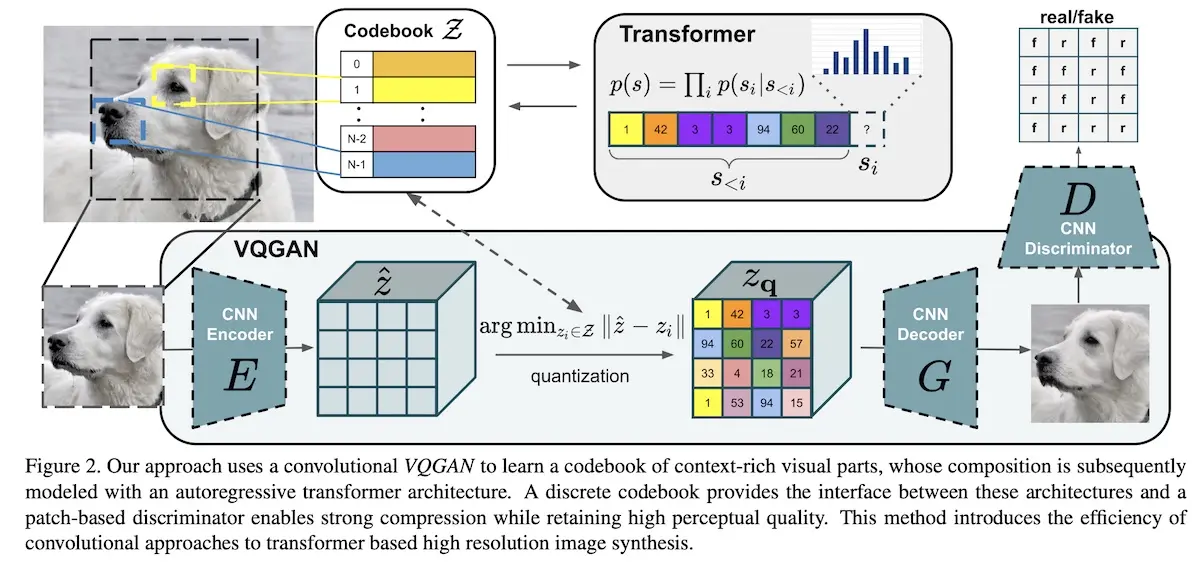
Example of a visual codebook from the VQGAN paper (Note, this is not DALL·E; source)

Why compress images into tokens in a codebook? The authors explained that using pixels directly as image tokens would require too much memory for high-resolution images. As a result, model capacity is spent on high-frequency details (i.e., pixels) instead of low-frequency structure (i.e., lines) that make images visually recognizable. (This is the same reason Stable diffusion encodes images into the latent space before running diffusion.)

First, DALL·E trains a discrete variational encoder (dVAE) to compress 256 x 256 images into 32 x 32 image tokens (vocabulary size = 8,192). The parameters of the dVAE are then frozen when training the transformer.

Next, image captions are lowercased and truncated to a max length of 256 tokens before being encoded (vocabulary size = 16,384). The image tokens are then concatenated after the text tokens (example below).

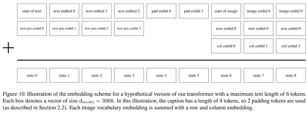
Example of concatenated text and image tokens in DALL·E (source)

Finally, an autoregressive transformer (i.e., predict the next item in a sequence) is trained to learn the joint distribution over the text and image tokens. The transformer is decoder-only, where each image token can attend to all text tokens earlier in the sequence.

To generate images from text, the text prompt is embedded and fed into the transformer. The transformer then generates the sequence of image tokens. Finally, the dVAE decodes the image tokens to return a 256 x 256 image.

DALL·E 2 (aka unCLIP, 2022) builds on the previous two papers by using the text and image encoder from CLIP and the autoregressive transformer from DALL·E. Similarly, unCLIP is trained on a dataset of image-caption pairs which are embedded via CLIP text and image encoders into text embeddings (\(z_{t}\)) and image embeddings (\(z_{i}\)).

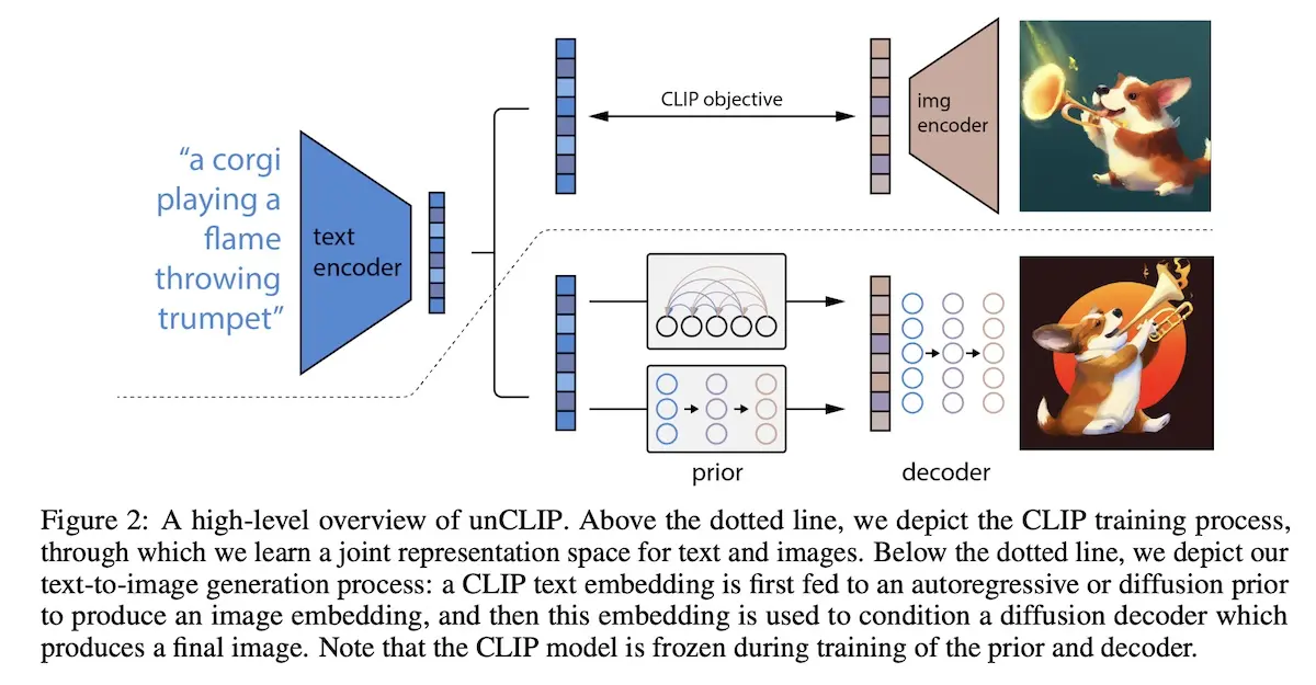
How the encoded text (blue) generates images via the prior and decoder (source)

In the image above, the prior (\(p(z_{i}\vert y)\)) learns to produce CLIP image embeddings (\(z_{i}\)) conditioned on the text prompt (\(y\)). The decoder (\(p(x\vert z_{i}, y)\)) then produces the image conditioned on the CLIP image embedding (\(z_{i}\)) and optional text prompt (\(y\)). In other words, to generate images from text prompts (\(p(x\vert y)\)), we first sample CLIP image embeddings via the prior before decoding them via the decoder.

The paper shared two approaches to learn the prior: autoregressive and diffusion.

The autoregressive approach is similar to that of DALL·E where text conditioning is done by having the text embedding early in the sequence. They also prepend a dot product token (of text and image embedding) between the text and image embedding. This allowed the autoregressive prior to condition the model on the higher dot product since a higher text-image dot product indicates images that are more representative of the caption.

For the diffusion approach, they trained a decoder-only transformer with a casual attention mask on a sequence of encoded text, text embedding, time step embedding, noised CLIP image embedding, and final embedding. The final embedding’s output is then used to predict the unnoised CLIP image embedding. Interestingly, in contrast to DDPM, they found it better to train the model to directly predict the unnoised image, instead of predicting the noise and then subtracting from the noisy image.

The latter shows one way text conditioning can be applied to diffusion. The transformer attends to the text information in the sequence and uses it to predict the final output.

Imagen (2022) takes it further by using a text encoder that wasn’t even trained on image-caption pairs (🤯). It uses the encoder network of the T5. This is a departure from CLIP-based approaches, where the text encoder is specifically trained on image-caption pairs and the text embeddings are projected into a multi-modal embedding space.

It works because extremely large language models (LLMs), by virtue of sheer size, can still learn useful representations despite not being explicitly trained on text-to-image tasks. The benefit is that LLMs can learn on a text-only corpus which is easily larger than image-text datasets. Furthermore, they found that scaling the text encoder size is more impactful than UNet size in image-text alignment and image fidelity.

Text encoder size > UNet size; dynamic thresholding > static thresholding (source)

Imagen does text conditioning by first tokenizing the input text and encoding it via the T5 encoder. The encoded text then passes through a pooling step (image below).

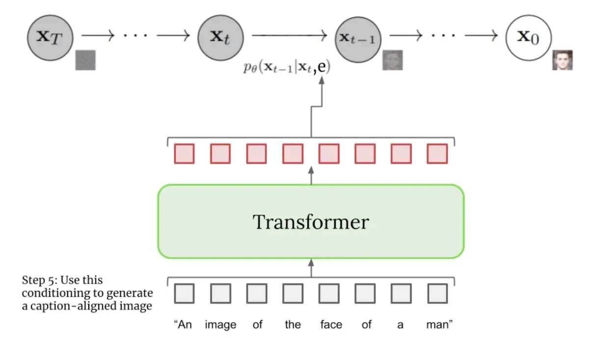
Encoding text via the T5 transformer in Imagen (source)

The text embedding is then combined with the image and time step embedding (image below). The model is conditioned via cross-attention over the text embedding. This is implemented by concatenating the text embedding to the key-value pairs of each self-attention layer in the UNet. Cross-attention on the text embedding outperformed simple mean or attention-based pooling.

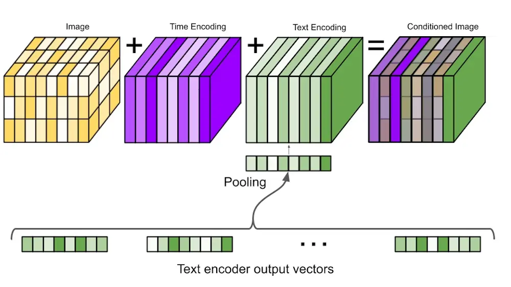
Conditioning on time and text embeddings in Imagen (source)

(Note how text is conditioned differently in DALL·E variants and Imagen. In DALL·E, text conditioning is done by concatenating the text embedding to the image embedding and then passing it through a transformer. In Imagen, text conditioning is done via cross-attention in the UNet.)

The text embedding (green and red boxes below) is used throughout the image generation step. First, it’s used to generate the initial 64 x 64 image from noise (blue box). Then, it is used to increase the image resolution to 256 x 256 and then 1,024 x 1,024 (yellow boxes).

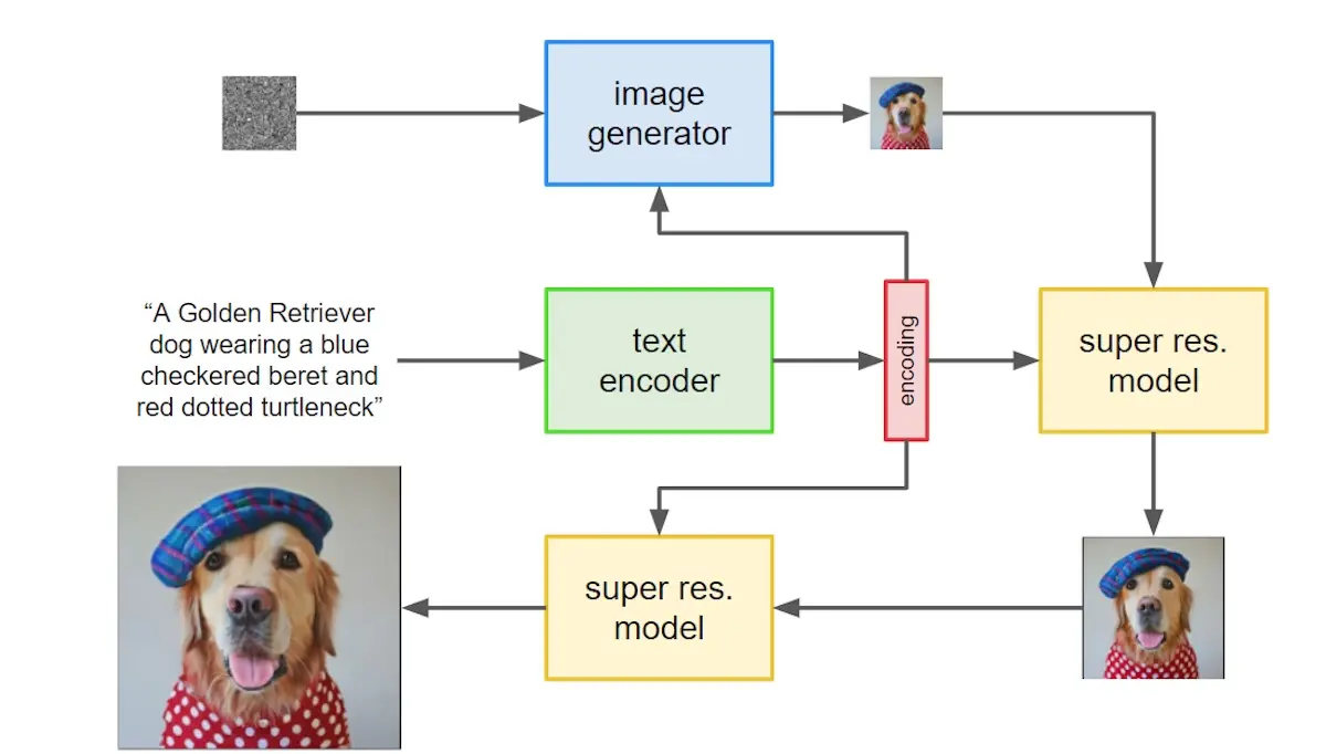
High-level overview of Imagen's text encoder, diffusion generator, and resolution model (source)

With text conditioning, we can now generate images based on text prompts. But text conditioning alone is insufficient to generate high-quality images that adhere to the text prompt—we also need guidance.

Classifier guidance: Increasing the strength of prompts

Guidance is a technique to explicitly incorporate image class—or text prompt—directly in the diffusion process. (This is the often tweaked guidance_scale hyperpameter.)

The classifier-guidance paper (2021) noted that GANs relied heavily on class labels, often via class-conditioned normalization or discriminators with heads designed to behave like classifiers. This suggests that class information is crucial to the success of GANs for generation. So, to take a leaf from GANs, they use a classifier \(p_\phi(y\vert x)\) to improve image generation via diffusion.

As a result, \(\nabla_{x} \log p_\phi(y\vert x)\) is added to the score function, updating it from \(\nabla_{x} \log p_\theta(x)\) to \(\nabla_{x} \log p_\gamma (x\vert y) = \nabla_{x} \log p_\theta(x) + \gamma \nabla_{x} \log p_\phi(y\vert x)\), where \(\nabla_x \log p_\phi(y\vert x)\) is the gradient of the classifier and \(\gamma\) is the guidance scale.

(Note: For simplicity, I’ve dropped the \(t\) variable in the equations. In practice, text-to-image diffusion is also conditioned on time step which indicates the level of input noise.)

To achieve this, they train a classifier (\(p_\phi(y \vert x)\)) on noised images (\(x\)) and then use the gradient (\(\nabla_{x} \log p_\phi(y \vert x)\)) to guide the sampling process towards the class label (\(y\)). To produce noised images, forward diffusion is applied on ImageNet with random crops to reduce overfitting. The classifier adopts the downsampling truck of the UNet, with pooling on the 8 x 8 layer to produce the final output.

Recall that the score function is now \(\nabla_x \log p_\gamma (x\vert y) = \nabla_x \log p_\theta(x) + \gamma \nabla_x \log p_\phi(y \vert x)\) and \(\gamma\) is the guidance scale. The paper found that increasing the guidance scale beyond 1 had the effect of amplifying the conditioning signal (i.e., text prompt) and led to better images.

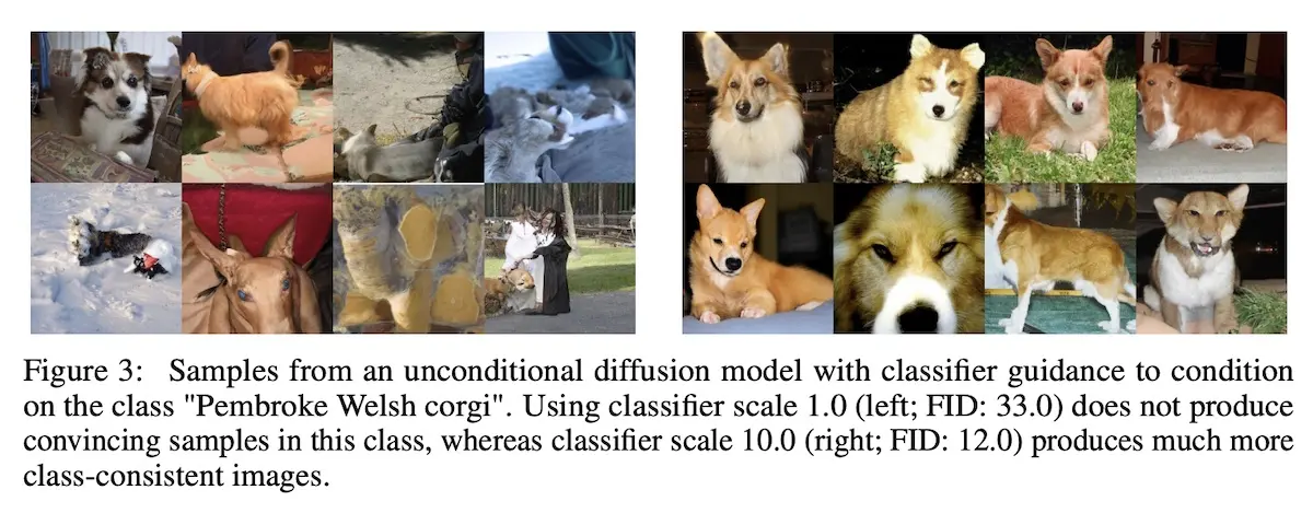
With standard (left; scale=1) and stronger (right; scale=10) classifier-guidance (source)

When using a scale of 1, while the classifier assigned reasonable probabilities of ~50% to the classes of the sampled images, upon visual inspection, these images did not match the classes. Scaling up the classifier gradients (i.e., guidance > 1) solved this issue and the class probabilities of the classifier increased to nearly 100%.

However, classifier guidance is impractical as the classifier needs to be trained—from scratch—on noisy images. I.e., we can’t use a pre-trained classifier.

Thus, classifier-free guidance (2021) was proposed. Instead of training a separate classifier, it trains a conditional diffusion model (\(p(x \vert y)\)) with conditioning dropout. Some proportion of the time, the conditioning information (i.e., image caption) is replaced with a null token. This is simple to implement and does not complicate the training pipeline or increase model parameters.

As a result, the single neural network can function as either a conditional model \(p(x|y)\) or unconditional model \(p(x)\), depending on the guidance scale:

• \(\gamma = 0\): unconditional model
• \(\gamma = 1\): standard conditional model
• \(\gamma > 1\): strongly conditional model that adheres more to the conditional (i.e., text prompt) and returns images with better text-alignment

GLIDE (2021) explored using both CLIP-guidance and classifier-free guidance. CLIP guidance was implemented by replacing the classifier with a CLIP model trained on noised images. They found that users preferred images generated via classifier-free guidance.

“A stained glass window of a panda eating bamboo”: No guidance (left) vs. CLIP-guidance (middle) vs. classifier-free guidance (right) in GLIDE (source)

To be clear, DALL·E, DALL·E 2, and Imagen apply classifier-free guidance too. DALL·E randomly drops the text-conditioning 10% of the time while DALL·E 2 randomly sets the text embeddings to zero and randomly drops text captions 10% and 50% of the time. Imagen randomly sets text embeddings to zero for 10% of training instances. In the space of text-to-image diffusion, classifier-free guidance (aka conditioning dropout) is now as essential as dropout for regularization.

That said, it was another development that allowed regular users to hack text-to-image diffusion on their laptops—departure to latent space.

Latent space: Diffusion on latents instead of pixels

Stable Diffusion (2021) differs from the previous diffusion models by working in the latent space instead of pixel space. It first compresses images via a variational autoencoder (VAE) into a more efficient and lower dimensional latent embedding. Next, the diffusion model learns to generate latent (i.e., compressed) representations of images which are then decoded into images via the VAE decoder.

Similar to DALL·E and its visual codebook, latent space is motivated by the observation that most pixels in an image are imperceptible details that are semantically meaningless. However, because regular diffusion models are trained and evaluated in the pixel space, it leads to unnecessary computation and thus costly training and inference. Thus, the paper proposes diffusion on compressed images where the imperceptible details are excluded.

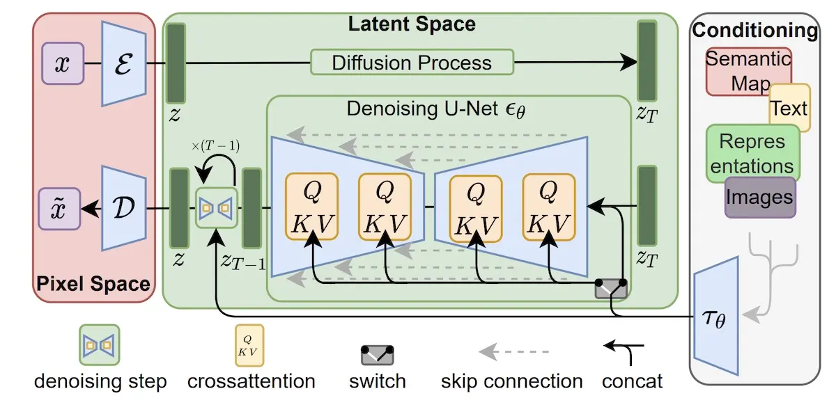
Using a VAE to encode images from pixel space to latent space (left) (source)

In Stable Diffusion, the VAE encodes noised images (via \(\mathcal{E}\)) into a low-dimensional latent representation which is fed into the UNet. It then decodes UNet-generated latent representations (via \(\mathcal{D}\)) into human-understandable images. The VAE has a reduction factor of 8, where the original image pixel space of 3 x 512 x 512 is encoded into latent space of 6 x 64 x 64, thus requiring 1/8 x 1/8 = 1/64 of the memory. During sampling, only the VAE decoder is needed.

Stable Diffusion uses the CLIP text encoder. (But as Imagen has demonstrated, probably any sufficiently large text-only LLM can be used).

Latent diffusion leads to faster training and sampling because we’re now working in the latent—instead of pixel—space. This leads to lower cost which leads to more experiments. The lower memory requirement also allows sampling run on consumer-grade laptops, putting text-to-image generation in the hands of regular hackers.

• • •

We started with how diffusion can generate images from noise. Then, we saw how text conditioning enabled prompt-based image generation via autoregressive transformers and cross-attention, even using text encoders that weren’t trained on text-to-image tasks. Finally, we learned how guidance helps with generating images that are more aligned with the text prompt though at the cost of image diversity.

The space of text-to-image has progressed rapidly since I started deliberately studying it. Two weeks ago, NVIDIA released eDiff-I which uses an ensemble of diffusion models. And we haven’t touched on text-to-video (e.g., Facebook’s Make-A-Video, Google’s Imagen Video) and text-to-3d (e.g., Google’s DreamFusion, NVIDIA’s Magic3D).

Unfortunately, we can’t discuss all of them here (mostly because I don’t have the spare time and energy 😅). Nonetheless, I hope these fundamentals will help with your understanding of text-to-media generation and its future advances.

Did I misunderstand or misrepresent any of the concepts or papers? If so, please reach out!

References

• Deep Unsupervised Learning using Nonequilibrium Thermodynamics
• Generative Modeling by Estimating Gradients of the Data Distribution (NCSN)
• Improved Techniques for Training Score-Based Generative Models
• Denoising Diffusion Probabilistic Models (DDPM)
• Denoising Diffusion Implicit Models (DDIM)
• Improved Denoising Diffusion Probabilistic Models
• Learning Transferable Visual Models From Natural Language Supervision (CLIP)
• Zero-Shot Text-to-Image Generation (DALL·E)
• Taming Transformers for High-Resolution Image Synthesis (VQGAN)
• Hierarchical Text-Conditional Image Generation with CLIP Latents (DALL·E 2)
• Photorealistic Text-to-Image Diffusion Models with Deep Language Understanding (Imagen)
• How Imagen Actually Works
• Exploring the Limits of Transfer Learning with a Unified Text-to-Text Transformer (T5)
• Diffusion Models Beat GANs on Image Synthesis (classifier-guidance)
• Classifier-Free Diffusion Guidance
• GLIDE: Towards Photorealistic Image Generation and Editing with Text-Guided Diffusion Models
• High-Resolution Image Synthesis with Latent Diffusion Models (Stable Diffusion)

If you found this useful, please cite this write-up as:

Yan, Ziyou. (Nov 2022). Text-to-Image: Diffusion, Text Conditioning, Guidance, Latent Space. eugeneyan.com. https://eugeneyan.com/writing/text-to-image/.

or

@article{yan2022diffusion,
  title   = {Text-to-Image: Diffusion, Text Conditioning, Guidance, Latent Space},
  author  = {Yan, Ziyou},
  journal = {eugeneyan.com},
  year    = {2022},
  month   = {Nov},
  url     = {https://eugeneyan.com/writing/text-to-image/}
}