RecSys 2020 ran from 22nd - 26th September. It was a great opportunity to peek into some of the latest thinking about recommender systems from academia and industry. Here are some observations and notes on papers I enjoyed.

Emphasis on ethics & bias; More sequences & bandits

There was increased emphasis on ethics and bias this year. Day 1’s keynote was “4 Reasons Why Social Media Make Us Vulnerable to Manipulation” (Video) while Day 2’s keynote was “Bias in Search and Recommender Systems” (Slides).

Two (out of nine) sessions were on “Fairness, Filter Bubbles, and Ethical Concerns” and “Unbiased Recommendation and Evaluation”, discussing papers such as:

• Deconstructing the Filter Bubble: User Decision-Making & Recommender Systems
• Debiasing Item-to-Item Recommendations with Small Annotated Datasets
• The Connection Between Popularity Bias, Calibration, and Fairness

Inverse propensity scoring was a popular approach taken to debias recommendations:

• Unbiased Learning for the Causal Effect of Recommendation
• Doubly Robust Estimator for Ranking Metrics with Post-Click Conversions
• Unbiased Ad Click Prediction for Position-aware Advertising Systems

We also saw an increased shift towards sequence models (with SASRec (2018) and BERT4Rec (2019) being common benchmarks) and bandit and reinforcement learning for recommender systems:

• SSE-PT: Sequential Recommendation via Personalized Transformer
• FISSA: Fusing Item Similarity Models with Self-Attention Networks
• Contextual User Browsing Bandits for Large-Scale Online Mobile Recommendation
• Learning to Collaborate via Multi-Agent Reinforcement Learning

Notable: Offline evaluation, MF > MLP, applications

Several papers on offline evaluation highlighted the nuances and complexities of assessing recommender systems offline and suggested process improvements. Also, Netflix gave a great talk sharing their findings from a comprehensive user study.

There was also a (controversial?) talk by Google refuting the findings of a previous paper where learned similarities via multi-layer perceptrons beat the simple dot product.

Of course, I also enjoyed the many papers sharing how organizations built and deploy recommender systems in the wild (more here).

User research on the nuances of recommendations

Zach Schendel from Netflix discussed recommendation complexity and their findings from user research. There are three sources of recommendation complexity, namely:

• Placement: Where is the recommendation located on the user interface?
• Person: Who is seeing the recommendation? What are her past experiences with the recommendation placement?
• Context: What is going on at that moment? What are the user’s needs?

Netflix found that users have different expectations across different recommendation placements. For example, users have higher expectations of similarity when it’s a 1:1 recommendation (e.g., after completing a show, Netflix would recommend a single next title). Such recommendations are risky as there are no backups, and there are no other recommendations to help the user understand similarity.

In contrast, users have lower expectations in 1:many recommendations (e.g., a slate of recommendations), such as when the user is browsing. In the example below, “Queer Eye” might seem far removed from “Million Dollar Beach House”. But with the other recommendations in the slate, it makes sense within the overall theme of reality shows.

They also found that users have higher expectations in recommendations that result from explicit actions (e.g., search). In general, the greater the user effort (e.g., search, click), the higher the user expectation. Contrast this to lower effort recommendations, such as on the home page, or in recommendation slates when casually browsing.

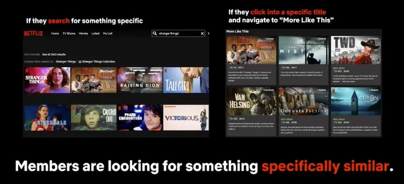
The two findings suggest there’s no one-size-fits-all approach for recommendations. Recommenders developed for the home page/email (low user effort) might not work similarly if placed on the detail page or search page. Also, 1:1 and 1:many recommendations should be built and evaluated differently.

Netflix also highlighted the importance of understanding users’ context. After finishing a reality show, users are likely to watch another reality show, right? Not necessarily. Netflix found that consecutive reality show watching happened only 18% of the time.

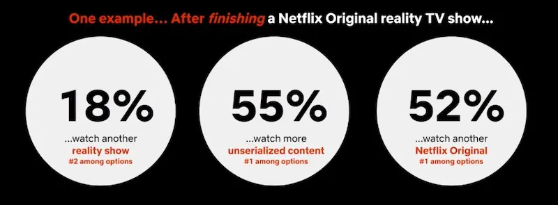
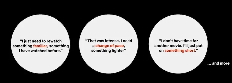
There are many contexts where similarity is not required or can worsen recommendations. For example, users might want a change of pace or mood from that horror movie they just watched. Also, does the user stick to a specific genre (e.g., Korean dramas) or hop around diverse genres? A better understanding will help improve the user experience.

Towards more robust offline evaluation and study reproducibility

Pablo Castells from the Autonomous University of Madrid shared about how different target sampling approaches affect offline evaluation. There are three ways of creating validation targets: With no unrated data, with all unrated data, and somewhere in between.

Three ways to generate validation set targets.

The relative performance of recommenders could differ based on how the validation set was created. Here’s an example below. On the left (with unrated data), recommendation set A outperforms recommendation set B. But on the right (without unrated data), recommendation set B is superior.

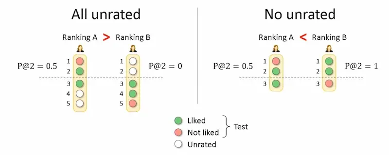
The relative performance of models differ when considering all unrated vs. no unrated labels.

They also ran several experiments on the MovieLens 1M dataset and demonstrated that the relative precision@10 performance differs with and without unrated data.

The relative performance of recommenders differ with and without unrated data.

Similarly, Zaiqiao Meng from the University of Glasgow showed how different data splitting strategies (for train and validation) can affect the relative performance of recommendation systems in offline evaluation. First, they discussed the four main data splitting strategies:

• Leave-one-last: Leave one last item, leave one last basket/session
• Temporal: Temporal split within each user, temporal split (on same date) globally
• Random: For each user, split interactions into train and test data
• User: Split some users into train, the rest into test

Then, with the three most popular splitting strategies (i.e., leave one last item, leave one last basket, and global temporal split), they ran experiments on the Ta Feng and Dunnhumby datasets. The relative performance of recommenders changed often across splitting strategies (indicated by the rank swaps).

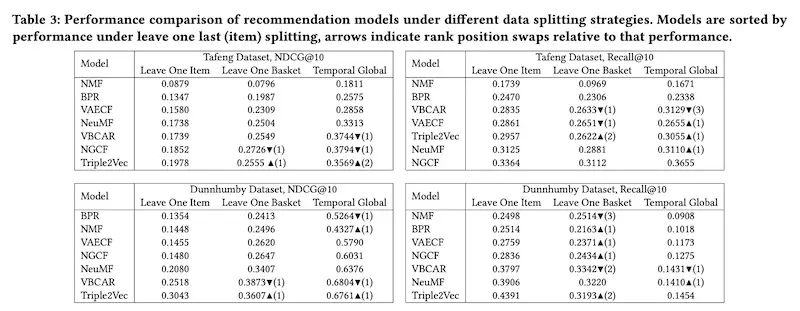
They also found certain models to perform better under different splitting strategies: Triple2vec performs better under leave one last item while VBCAR does better under temporal evaluation.

Zhu Sun from Macquarie University examined 85 papers on implicit feedback-based top-N recommendations published in the past three years. Their paper gave a good overview of the different factors that could affect recommendation systems such as data pre-processing (and how data is excluded), objective functions, negative sampling, data splitting approaches, and evaluation metrics.

Among the 85 papers, they found inconsistencies on:

• Data filtering: Some studies excluded users and items with less than 5 ratings while others used a threshold of 10.
• Validation: Some used leave-one-out, others used split by ratio. (They also found 37% of papers tuned hyperparameters on the test set!)
• Negative sampling: Approaches included uniform sampling, low-popularity sampling, and high-popularity sampling.

Unsurprisingly, the relative performance of various models differed with different combinations of pre-processing, negative sampling, evaluation metrics, etc.

Pigi Kouki from Relational AI highlighted one key failing in offline evaluation metrics: They penalize a model if it does not predict the same product (i.e., identical product ID). Thus, near-identical products—which a human might consider relevant—are not counted as hits. She then shared about their two-step offline evaluation process when building a recommender system.

First, they trained 15 models and selected five which performed best in offline evaluation:

• SR-GNN: Best hit rate, mean reciprocal rank, and nDCG
• V-STAN: Best precision, recall, and mean average precision
• V-SKNN, GRU4Rec: Best coverage and popularity
• STAMP: Satisfactory in all metrics

In the second step, human experts evaluated the recommendations from the five models. 10 experts evaluated the model across three categories in the home improvement domain. The experts had access to title, description, image, and links to the product. They could rate the recommendation as objectively relevant 👍, subjectively relevant ✅, or irrelevant 👎.

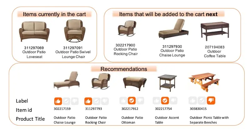
Recommendations were evaluated as objectively relevant 👍, subjectively relevant ✅, or irrelevant 👎.

In contrast to the offline evaluation metrics, human experts found GRU4Rec to have very relevant recommendations. However, because its recommendations did not match the IDs of products added to cart, GRU4Rec did not perform as well on offline evaluation metrics.

STAMP and GRU4Rec performed best in the second step and STAMP was put through an A/B test. This led to a 15.6% increase in CTR and an 18.5% increase in revenue per session.

Overall, these papers made me rethink my experimentation and offline evaluation workflow. Furthermore, offline evaluation of interactive machine learning systems (e.g., recommendation, search) is tricky as we can’t observe how user behaviour will change.

Comparing the simple dot-product to learned similarities

Walid Krichene from Google revisited (and overturned) the findings from the neural collaborative filtering (NCF; 2017) paper in his talk Neural Collaborative Filtering vs. Matrix Factorization Revisited.

In the original NCF paper, a multi-layer perceptron (MLP) was suggested to replace the dot product. This was based on experimentation results (where MLP was superior) and the universal approximation property.

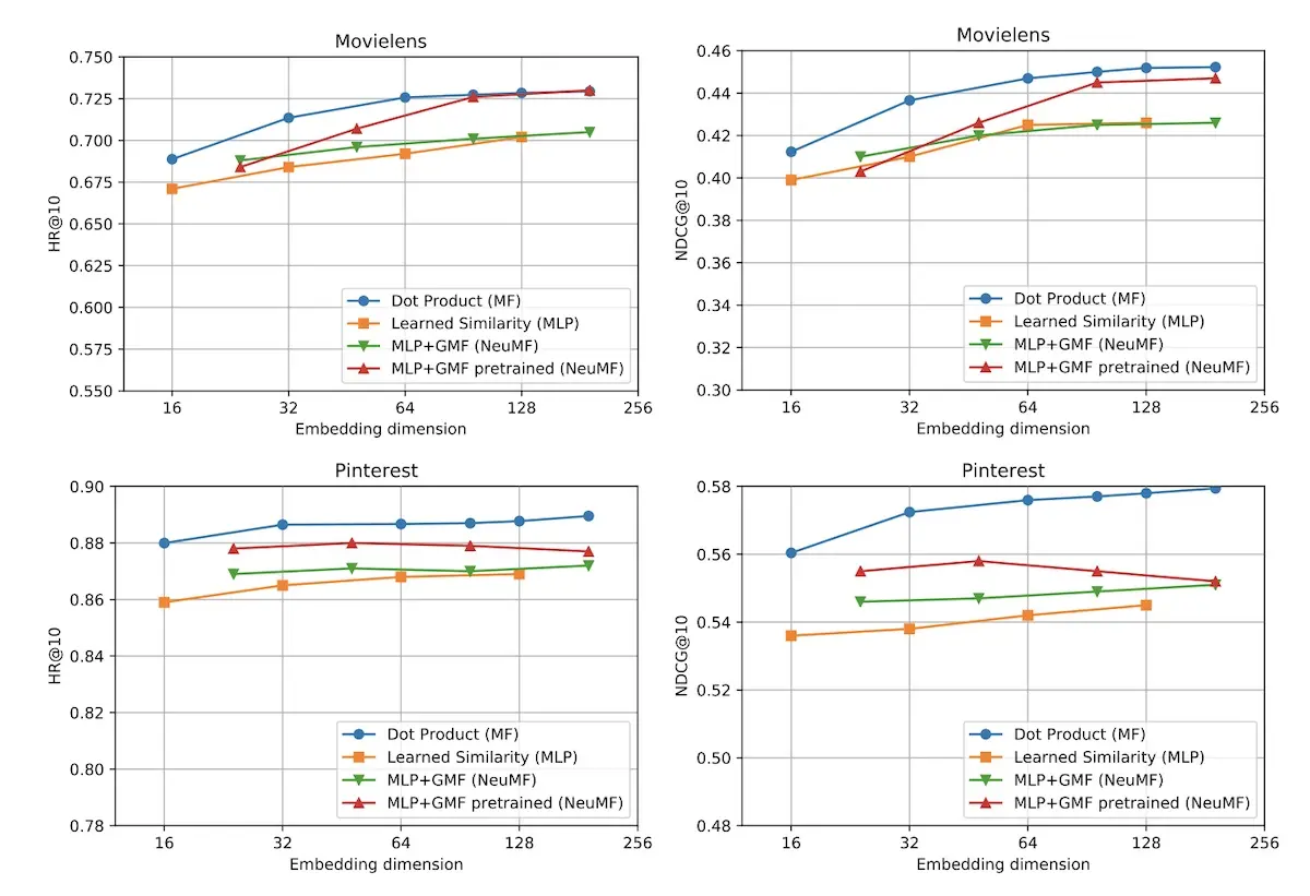
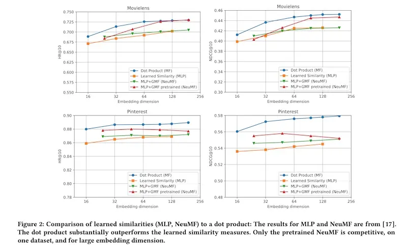
For the current paper, the team ran multiple experiments on the MovieLens 1M and the Pinterest dataset. They found the dot product to be superior to learned similarity approaches (MLP and neural matrix factorization).

When asked, Walid suggested that one possible reason was better hyperparameters. They found the matrix factorization parameters in the original NCF paper under regularized. Another possible reason could be the addition of explicit biases that have been empirically shown to improve model performance.

The paper also highlighted the practical advantages of the dot product, where retrieval can be done efficiently (linear complexity vs quadratic complexity for MLP). The dot product also doesn’t need to be learned. Thus, for most applications, the dot product should be the default approach.

(Note: In a previous paper, Google had also demonstrated that MLPs/feed-forward networks were inefficient in capturing multiplicative interactions.)

Industry applications: context, unexpectedness, interesting use cases

Moumita Bhattacharya from Etsy shared about their two approaches to integrate search query as context into their content-based recommender (image below). The goal is to include user intent (i.e., search query) and seasonality in candidate generation.

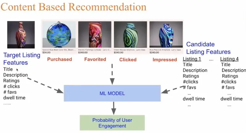
Etsy's content based recommender (without context).

For their first approach, they extracted top N queries associated with each listing and then trained embeddings for items and queries. With these embeddings, candidates were generated via approximate nearest neighbours. However, this did not work as well as the second, simpler approach.

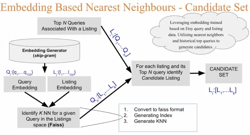
Etsy's first approach to context-based candidate generation.

Here’s their second approach: For each search query, a set of items would be shown to the user (i.e., search results)—these are the target items. Then, for each target item, other items the user interacted with (in the same search session) become candidate items. Thus, for each query-target pair, they would have a set of candidates.

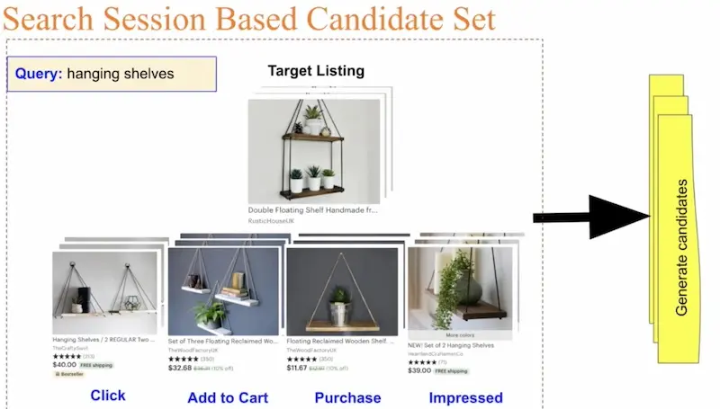
Etsy's second approach to context-based candidate generation.

Together with a ranker (applied after candidate generation), they improved recall by 12.42% in offline evaluation. In online evaluation, it increased click-through rate by 8 - 23% and conversion rate by 0.25 - 1.16%.

Casper Hansen from the University of Copenhagen shared how Spotify learns user preferences based on session history and the current context. Specifically, by using the sequence of past sessions and the context (at the start of each session), can they predict which tracks will be played in a new session and context?

Users played music in a variety of contexts (time, device).

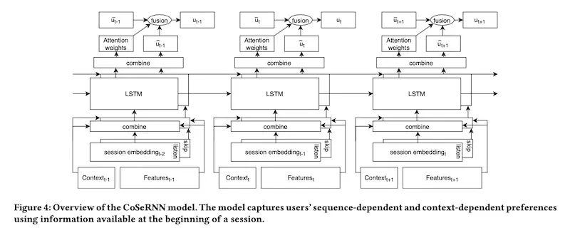
Music track embeddings (40-dimension vectors) were trained via word2vec. Then, track embeddings were averaged to create three session embeddings (all tracks, played tracks, skipped tracks). Context was represented via categorical variables such as day of week, time of day, device, etc.

They used an RNN-based architecture to jointly learn from historical sequences and context. The key was to fuse the context-dependent user embeddings and long-term user embeddings using attention weights.

Pan Li from New York University shared how Alibaba’s Youku introduces freshness and unexpectedness into video recommendations. He distinguished between two kinds of unexpectedness:

• Personalized: Some users are variety seekers and thus more open to new videos
• Session-based: If a user finishes the first episode of a series, it’s better to recommend the next episode. If the user binged on multiple episodes, it’s better to recommend something different.

Their final utility function combines relevancy (i.e., CTR) and unexpectedness. The proportion of unexpectedness is tuned to ensure that CTR is kept at a certain threshold while introducing unexpectedness.

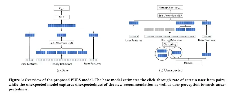
Two separate models were implemented, one for relevancy and one for unexpectedness.

Results from an A/B test showed an increase in number of videos viewed by each user (3.74%), time spent on platform (4.63%), and CTR (0.80%) while also increasing unexpectedness by 9.74%.

Benjamin Chamberlain from Twitter shared how it’s a bad idea to use default parameters for Word2vec-based recommendations. They quantified the extent of this with experiments on hyperparameter tuning and evaluated on recall@10 and nDCG@10.

Under constrained optimization (i.e., considering limited resources), they got a 138% average improvement in recall (aka hit rate; results below). And by tuning on a 10% data sample, they achieved a 91% average improvement in recall. From these experiments, they increased follow rates from Twitter’s Who To Follow recommender by 15%.

Ehtsham Elahi from Netflix shared how to learn representations of recommendation slates. A slate is a row of recommendations, such as what you would see on the Netflix home screen. In recommendations, we’re often recommending and ranking slates of items instead of individual items.

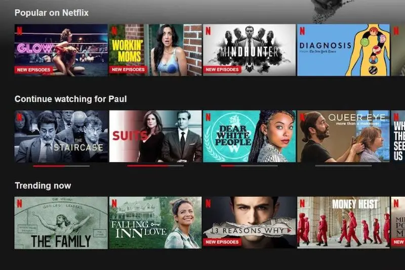
Recommendation slates on Netflix's home screen.

They demonstrated a way to learn state embeddings by using the distribution of items making up the slate. This is done by summarizing the items in the slates using the mean and covariance matrix of the item embeddings.

By incorporating slate embeddings, they improved on the winning submission for the RecSys 2019 challenge (predicting accommodations clicks in Trivago search results).

Ramanathan R from SBX Corporation shared their approach for building a reciprocal recommender system for a matchmaking app. Recommendations for matchmaking are challenging for the following reasons:

• A successful match requires both parties to like each other; in product recommendations, we only need to model one-sided preferences
• Once a match is made, most matched users will stop using the app and thus exclude themselves from the candidate pool
• The dataset is very sparse as users are selective and thus have few interactions
• Too many poor recommendations can lead to high rejection rate and user attrition

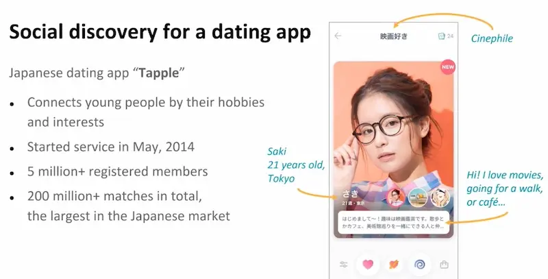
Data available from Tapple's matchmaking app.

To learn user embeddings, they used historical match data. If both users liked each other (i.e., match), this was assigned a positive label; if only one user liked (and the other user rejected or ignored), this was assigned a negative label. For new users, pseudo-embeddings were generated based on existing users with similar metadata (e.g., location, interests). These user embeddings were then used in candidate generation.

An interesting challenge was the mismatch between offline and online evaluation. This was due to some recommended users being inactive (e.g., previously matched or stopped using the app). Inactive users did not reciprocate the like, leading to no match/conversion. This was fixed by adding a re-ranking step to have a balance of relevant, new, and active users.

Thanks to Yang Xinyi and Karl Higley for reading drafts of this.

If you found this useful, please cite this write-up as:

Yan, Ziyou. (Sep 2020). RecSys 2020: Takeaways and Notable Papers. eugeneyan.com. https://eugeneyan.com/writing/recsys2020/.

or

@article{yan2020recsys,
  title   = {RecSys 2020: Takeaways and Notable Papers},
  author  = {Yan, Ziyou},
  journal = {eugeneyan.com},
  year    = {2020},
  month   = {Sep},
  url     = {https://eugeneyan.com/writing/recsys2020/}
}