Spark+AI Summit 2020 took place on 24-26 June. I’m only halfway through and it’s filled with gems of practical knowledge.

Figuring out which talks to attend can be overwhelming though. For example, 24th June has close to 100 sessions, not including keynotes and forums. ctrl+f on the following gives us the following matches:

• “beginner”: 4
• “intermediate”: 56
• “advanced”: 7
• “sponsored”: 24
• “ask me anything”: 6

Most people don’t have the time to sift through and attend these talks. Thus, I’m tidying up my notes and sharing a high-level summary on selected talks. This write-up will focus on the application-agnostic talks; the next one will be application-specific.

Table of Contents

• Scaling Up Deep Learning By Scaling Down
• How (Not) To Scale Deep Learning in 6 Steps
• Scaling AI Research to Production with PyTorch
• Probabilistic Data Structures For Humans
• Improving Broadcast Joins In Apache Spark

Scaling Up Deep Learning By Scaling Down (24th June)

Nick Pentreath, Principal Engineer at IBM’s Center for Open Data and AI, shares four ways to improve model training and performance efficiency.

Architecture improvements: Inception V3 uses the standard convolution block and has 24 million parameters. In contrast, MobileNet V1 uses depth-wise convolution blocks and has only 4 million parameters. However, accuracy also suffers (78.8% vs 70.9% on ImageNet).

Trends in deep learning are changing. In the past, CNN models focused on accuracy (getting higher on the y-axis). Recently, the focus has shifted towards accuracy and efficiency (keeping the x-axis and the size of the models low).

Initially, models were moving to the top-right; now, the focus is on the top-left and keeping them small

Google also shared about EfficientNet which use neural architecture search to find optimal architectures. However, searching for the right architecture consumes a lot of resources.

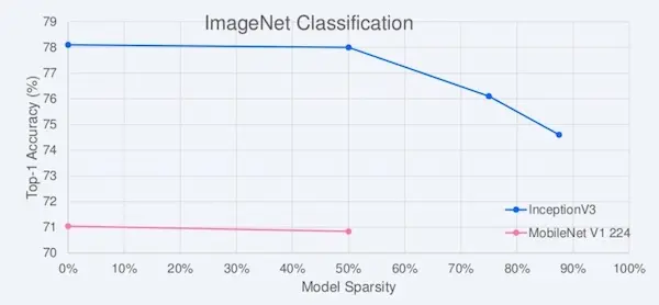
Model pruning. Many of the weights in a neural network are not used. Here’s example of how we could prune as much as half the weights in InceptionV3 and MobileNet V1 with minimal loss in accuracy on ImageNet.

Half of the weights can be pruned with minimal performance loss

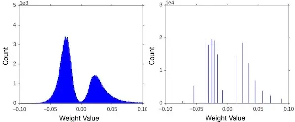
Quantization. We can reduce the numerical precision of weights by binning the values (i.e., reducing from 32-bit to 16-bit while still retaining the histogram distribution).

The distribution of weights can be retained at lower precision

Quantization has two flavours: post-training and training-aware. Post-training quantization avoids retraining a model again, but there’s some drop in accuracy (77.2% vs 63.7%). Training-aware quantization is more complex though it has lesser accuracy loss (77.5% vs 70.9%)

Model distillation. From the examples on pruning, it’s clear that our large neural networks are usually over parameterised. One way to slim them down is to train a smaller (student) model to mimic the larger (teacher) model’s predictions.

A distilled (student) model can be trained on the teacher model's output, and ground truth labels

The smaller model can be trained on both the teacher’s soft-labels and the ground truth labels. The soft-labels usually have higher entropy and provide more information and less variance. Thus, the smaller model can be trained on less data at a higher learning rate.

In some cases, the distilled model is stronger than the original model, providing higher accuracy and efficiency (further demonstrating that most models are over-parameterised). Some successful distilled models include DistilBERT and TinyBERT.

Further Reading:

• Scaling Up Deep Learning By Scaling Down Slides
• Benchmark Analysis of Representative Deep Neural Network Architectures
• To prune, or not to prune: exploring the efficacy of pruning for model compression
• Deep compression: Compressing deep neural networks with pruning, trained quantization and Huffman coding.
• Distilling the Knowledge in a Neural Network

How (Not) To Scale Deep Learning in 6 Steps (24 June)

Sean Owen, Principle Solutions Architect at Databricks, shares 6 tips on how to scale the training of deep learning models, in the following order:

These steps use a 10% sample of the data for quick experimentation and iteration (Step 0 is “Use a sample and work in memory”):

• Use a GPU: Cloud makes access to this easy
• Use early stopping: In the example provided, this reduced training time from 60 minutes to 18 minutes, with better accuracy (76% vs 76.7%).
• Use larger batch sizes to max out the GPU: This further reduced training time to 9 minutes with similar accuracy (76.3%)

These steps use the full data set to optimize for model performance:

• Use Petastorm to iterate over large data: Petastorm was designed by Uber to iteratively feed Parquet-based data into deep learning frameworks (initially TensorFlow, now supports PyTorch too) almost as efficiently as in memory. While we’re using 10x the data, epoch times are only 11x longer. Accuracy goes up to 83%.
• Use multiple GPUs: Most modern deep learning frameworks allow the use of multiple GPUs with minimal code changes.
• Use Horovod across multiple machines: If multiple GPUs on a single machine isn’t enough, consider using Horovod which helps to scale training on GPUs across multiple machines.

Further Reading:

• How (Not) To Scale Deep Learning in 6 Easy Steps
• Meet Horovod: Uber’s Open Source Distributed Deep Learning Framework for TensorFlow (Now works with PyTorch too, yay!)

Scaling Research to Production with PyTorch (26 Jun)

Joe Spisak, PyTorch Product Lead at Facebook, drops knowledge on PyTorch and its ecosystem that helps simplify the training and deployment of models at scale.

To reduce model size and computation requirements, PyTorch comes with in-built model pruning and quantization. Facebook has been deploying quantized models for years and it helps with inference at scale, especially on model devices.

To train models at scale, there’s TorchElastic. It enables distributed PyTorch jobs in a fault-tolerant and elastic manner. This ensures that jobs don’t get disrupted when machine(s) go down, or when your AWS spot instance gets outbid.

To deploy models at scale, there’s TorchServe which was jointly developed with AWS. It makes it easy to achieve lightweight serving, provides default handlers for common tasks, model versioning for A/B testing, etc.

Further Reading:

• Introducing TorchServe: a PyTorch model serving framework
• TorchElastic on GitHub
• TorchServe on GitHub

Probabilistic Data Structures For Humans (25 June)

Yeshwanth Vijayakumar, Project Lead/Architect at Adobe, shares about three probabilistic data structures for quick queries on large datasets. These data structures work because they’re monoids. Wait, what are monoids?

Here’s a simplified explanation. Monoids have the following properties:

• Can be combined with other values (of the same type) to form new values (of the same type): int(1) + int(2) = int(3)
• Operations are associative (order doesn’t matter): 1 + (2 + 3) = (1 + 2) + 3
• They have an identity value: 1 + 0 == 1, where 0 is the identity value

Bloom filters check for membership in a probabilistic way (e.g., set.exist(item)). They can be used to answer questions like: Has the user viewed this product before?

If the result is False, then the item definitely does not exist in the set. If the result is True, there’s a possibility that the item does not exist in the set.

HyperLogLog counts the number of distinct elements in a set (e.g., set.count_distinct()). This can be used to answer questions like: How many unique users bought items A, B, and C?

Because HyperLogLog is a monoid, we can count the number of unique users for each product, then perform a union across all the products.

Count-min sketch can be thought of as a frequency table of events in a stream of data. This can be used to answer questions like: How many items did this seller transact today?

It uses hash functions to map events to frequencies—thus, it uses sub-linear, instead of O(n), space. However, because it uses a hash function, it could over count some events due to collisions.

Further Reading:

• Monoids
• Count-min Sketch
• Why Spark Can’t Fold Left

Improving Broadcast Joins In Apache Spark (25 June)

Jianneng Li, Software Engineer at Workday, shares practical insight and experiment results from optimising broadcast joins.

Is the broadcast join always faster (if the data can fit into memory)? Not necessary. There’s significant overhead to broadcast joins, which includes:

• Collecting the broadcasted table (on the driver)
• Building the hash table (on the driver)
• Sending the hash table to the executor
• Deserializing the hash table (on the executor)

What’s the I/O cost difference between the (regular) sortMergeJoin and the broadcastHashJoin? Let’s assume we have two tables: A is the bigger table and B is the smaller table to be broadcasted. We also have n cores.

For sortMergeJoin (SMJ), the total I/O cost is 3(A/n) + 3(B/n):

• On A: Read (A/n), Sort, Write (A/n)
• On B: Read (B/n), Sort, Write (B/n)
• Join: Read (A/n, Read(B/n), Join

For broadcastHashJoin (BHJ), the total I/O cost is: A/n + B/n + 2B:

• On B: Read (B/n), Build hash table, Write (B)
• Join: Read (A/n), Read (B), Join

Simplifying the above, the cost difference between both SMJ and BHJ is 2(A + B)/n - 2B. We can further simplify this by considering A as a magnitude of B: If A has 10 million rows and B has 2 million rows, then B = 1 and A = 5. Thus, the cost difference between SMJ and BHJ is (A+1)/n.

When (A+1)/n is less than 1 (i.e., you have many cores), then SMJ will be faster. But if (A+1)/n is much greater than 1 (i.e., your left table is much bigger than the right, broadcasted table), then BHJ will be faster.

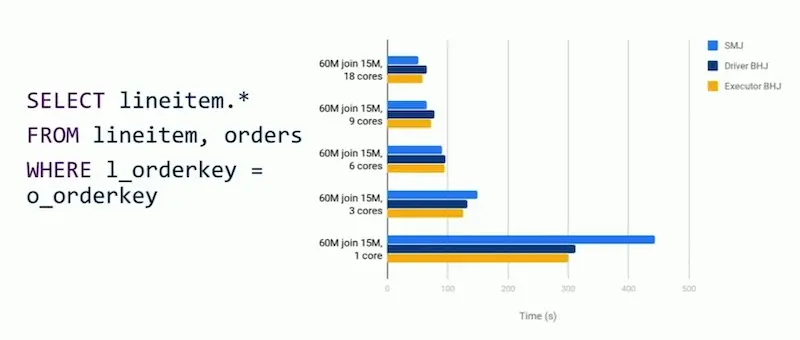
In an experiment where A = 60 million and B = 15 million (thus A+B = 5), we see that with more than 5 cores, SMJ does better (i.e., lesser time). Otherwise, BHJ does better.

As the number of cores exceed 5, sort-merge join performs better.

Similarly, keeping n (number of cores) constant at 18, we see that BHJ outperforms SMJ when A+B exceeds 20.

As the left table A grows relative to the broadcast table B, broadcast-hash join performs better.

However, with automatic broadcasting (via adjusting the broadcast threshold), make sure the smaller table is on the right. Even when the smaller table is on the left, Spark will try to broadcast the bigger table on the right, leading to inefficiency.

Workday is currently working on executor-side BHJ (Spark currently has driver-side BHJ) which has shown tremendous improvement in broadcast performance (SPARK-17556). Hopefully, this will be merged soon.

Further Reading:

• Performance Tuning: Converting sort-merge join to broadcast join
• What is the Difference between Broadcast hash join and Broadcast Nested loop join?
• SPARK-17556 Executor side broadcast for broadcast joins

Eager to apply this practical knowledge

The practical knowledge from Spark+AI Summit 2020 is invaluable. I’m eager to apply it to my work on spark pipelines and deep learning. Next week, I’ll share some application-specific talks at the conference.

P.S., Are there any good sessions I missed? Let me know in the comments below =)

If you found this useful, please cite this write-up as:

Yan, Ziyou. (Jun 2020). My Notes From Spark+AI Summit 2020 (Application-Agnostic Talks). eugeneyan.com. https://eugeneyan.com/writing/notes-from-sparkai-summit-application-agnostic/.

or

@article{yan2020spark,
  title   = {My Notes From Spark+AI Summit 2020 (Application-Agnostic Talks)},
  author  = {Yan, Ziyou},
  journal = {eugeneyan.com},
  year    = {2020},
  month   = {Jun},
  url     = {https://eugeneyan.com/writing/notes-from-sparkai-summit-application-agnostic/}
}