NLP for Supervised Learning - A Brief Survey
It’s hard to keep up with the rapid progress of natural language processing (NLP). To organize my thoughts better, I took some time to review my notes, compare the various papers, and sort them chronologically. This helped in my understanding of how NLP (and its building blocks) has evolved over time.
To reinforce my learning, I’m writing this summary of the broad strokes, including brief explanations of how models work and some details (e.g., corpora, ablation studies). Here, we’ll see how NLP has progressed from 1985 till now:
- Sequential models: RNN (1985), LSTM (1997), GRU (2014)
- Word embeddings: Word2vec (2013), GloVe (2014), FastText (2016)
- Word embeddings with context: ELMo (2018)
- Attention: Transformer (2017)
- Pre-training: ULMFiT (2017), GPT (2017)
- Combining the above: BERT (2018)
- Improving BERT: DistilBERT, ALBERT, RoBERTa, XLNet (2019); Big Bird, Multilingual embeddings (2020)
- Everything is text-to-text: T5 (2019)
(Did I miss anything important or oversimplify? Any errors? Please reach out with suggestions and I’ll update. Thank you!)
Sequential models to process a sentences (1985)
Recurrent neural networks (RNNs) were first introduced around 1985 - 1986 (based on this thread). They differ from regular feedforward neural networks in that their hidden layers have connections to themselves. This allows them to operate over sequences (e.g., sentences of word tokens).
The state of the hidden layer at one time-step is used as input to the (same) hidden layer at the next time-step; thus the name “recurrent”. This allows the hidden layers to learn information about the temporal relationships between tokens in the sequence. For more details, check out Andrej Karpathy’s excellent post.
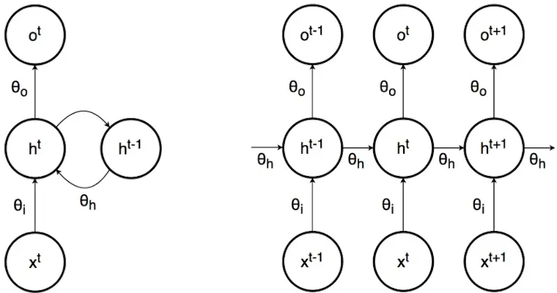
RNN (left) and its unrolled view (right) (source)
However, RNNs had difficulty with modelling long-range dependencies (e.g., words that are far apart in a long sentence) due to vanishing/exploding gradients. With long sequences, the product of partial derivatives (through backpropagation) becomes very small (i.e., vanish). This happens when the partial derivatives are < 1. The reverse occurs when the partial derivatives are > 1 and the product explodes.
The Long Short-Term Memory (LSTM) architecture introduced in 1997 improves on this. LSTMs model long-range dependencies better through gates:
- Forget gate: Decides what information, from the current input and previous hidden state, to forget (i.e., discard) via a sigmoid
- Input gate: Decides what information to remember (i.e., stored) via a sigmoid
- Output gate: Decides what the next hidden state should be
Together, these gates improve how the LSTM learns—what should be forgotten and what should be remembered? More details in Chris Olah’s explanation. Though the LSTM was introduced in 1997, it wasn’t until 2015 that they saw commercial use: Google Voice, Apple’s QuickType and Siri, Amazon’s Alexa, and Facebook’s automatic translations.
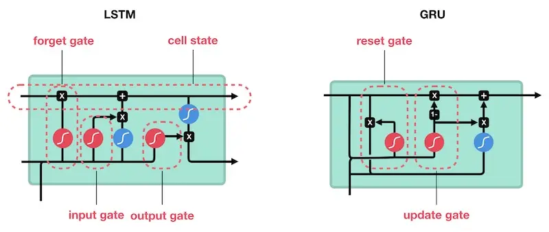
Comparison between the LSTM and GRU (source)
Gated Recurrent Units (GRUs) simplified the LSTM in 2014. It has only two gates, an update gate (similar to LSTM’s forget and input gate) and a reset gate (which also decides how much to forget). Because it has fewer gates (and thus fewer math operations), it’s faster to train. (In my work, I’ve found GRUs to converge faster with greater stability).
Word embeddings to learn from unlabelled data (2013)
In 2013, Word2vec (w2v) was introduced. Through unsupervised learning, it represents words as numbers, or more precisely, vectors of numbers. (Previously this was done via one-hot encoding). Being unsupervised, it’s able to learn on large corpora of unlabelled data (e.g., Wikipedia). When used in a variety of downstream tasks (e.g., classification), these word embeddings greatly improve model performance.
There are two ways to train w2v models: Continuous Bag of Words (CBOW) and Skip-gram. In CBOW, we predict the center target word given the context words around it. In Skip-gram, we predict the surrounding context words given a center word (similar to CBOW, but in reverse). Skip-gram was found to work better with smaller amounts of data and to represent rare words better. CBOW trains faster and has better representations of more frequent words. (I’ve usually found Skip-gram to work better.)
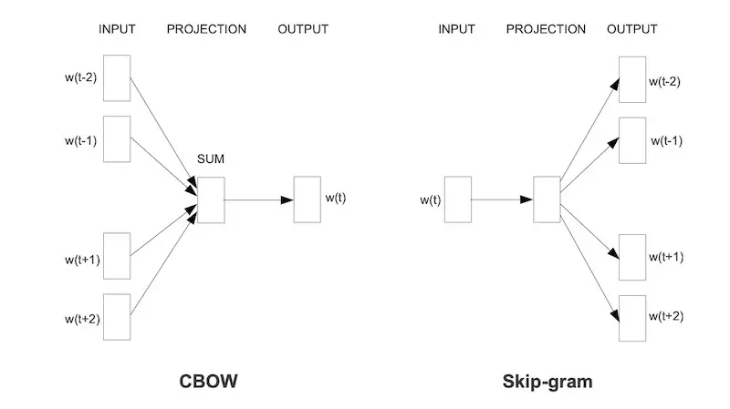
Continuous Bag of Words vs. Skip-gram (source)
Why does Skip-gram work better for rare words?
I've found this intuition helpful for understanding this. Let’s start with a sample sentence: “Today is a ___ day for writing”. The most common center words include “beautiful”, “productive”, “great” while rare words include “hellacious”.
In CBOW, the rare words (i.e, “hellacious”) are drowned out by the more frequent words. Thus, CBOW doesn’t learn representations of these rare words as well.
However, with Skip-gram, these rare words don’t have to “compete” with the more common words (in terms of probability of occurrence). Instead, they have their own context pairs, such as (“is”, “hellacious”), (“a”, “hellacious”), (“hellacious”, “day”), and (“hellacious”, “for”). These context pairs are treated as separate observations and thus help Skip-gram to learn these rare words better.
Word2vec applied subsampling, where words that occurred relatively frequently were dropped out with a certain probability. This accelerated learning and improved word embeddings for rare words.
It also tweaked the problem slightly. Instead of predicting the most probable nearby words (out of all possible words), it tries to predict whether the word-pairs (from skip-gram) were actual pairs. This changes the final layer from a softmax with all the words (expensive) to a sigmoid that does binary classification (much cheaper) .
However, our dataset and word pairs only have positive samples. Thus, negative sampling is done to generate negative samples based on the distribution of the unigrams. (In the paper, they applied an interesting trick and raised the word counts to the 3/4 power.)
Global Vectors for Word Representation (GloVe) was introduced a year later (2014). While w2v learns word co-occurrence via a sliding window (i.e., local statistics), GloVe learns via a co-occurrence matrix (i.e., global statistics). GloVe then trains word vectors so their differences predict co-occurrence ratios. Surprisingly, though w2v and GloVe have different starting points, their word representations turn out to be similar.
There are also variants of w2v that learn subword or character embeddings. Subword embeddings learn the most frequent character segments (i.e., breaking a word into 2-3 character segments). One approach is FastText (where the original Word2vec author is a co-author). FastText open-sourced its code as well as the multiple-language word embeddings trained with it.
What did we do before embeddings?
Before embeddings, we mostly relied on n-grams and one-hot vectors to represent text. (With embeddings, one-hot approaches are used less often. This occurs in non-NLP machine learning too, where categorical values are increasingly represented with embeddings instead of one-hot.)
On top of these one-hot vectors, we can apply singular vector decomposition (SVD) for topic modelling. Various supervised learning techniques (e.g., logistic regression, naive Bayes, decision trees, neural networks) can also be applied for classification (e.g., sentiment analysis, spam detection).
An example of this is the Otto Product Classification Competition on Kaggle. In this competition, the dataset had 93 numerical features that represented counts of different events. This is assumed to be counts of product text tokens and other attributes. The top submissions used TF-IDF and ensembles of decision trees, K-nearest neighbours, naive Bayes, and neural networks (more here).
For my product classification API, I adopted a combination of n-grams, TF-IDF, and naive Bayes. Paul Graham also used a similar approach for spam detection.
Improving word embeddings with context (2018)
In traditional word embeddings (e.g., Word2vec, GloVe), each token has only one representation (i.e., embedding). This is regardless of how it’s used in a sentence. For example, “date”:
- They went out on a “date”.
- What “date” is it today?
- She is eating her favourite fruit, a “date”.
- That photo looks “dated”.
Embeddings from Language Models (ELMo) improves on this (in 2018) by providing word representations based on the entire sentence. It does this via a bidirectional language model (biLM). ELMO’s biLM comprises a two-layer bidirectional LSTM.
By going both left-to-right (LTR) and right-to-left (RTL), ELMo can learn more about a word’s context. For example, in “Today is a hellacious day for writing”, the LTR LM will encode “today is a” while the RTL LM will encode “writing for day”. Together, they consider the entire sentence for the word “hellacious”. These embeddings are learned via separate LMs and concatenated before being used downstream. (Why do these LMs have to be separate? See Why can’t we use bidirectional context with multiple layers?)
Pre-trained ELMo can be used in a variety of supervised tasks. First, the biLM is trained and the word representation layers are frozen. Then, the ELMo word representation (i.e., vector) is concatenated with the token vector to enhance the word representation in the downstream task (e.g., classification).
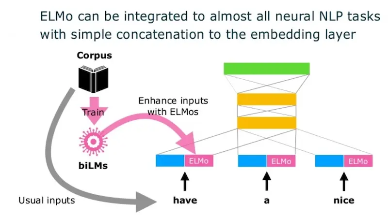
ELMo embeddings concatenated with input tokens (the blue blocks) for downstream tasks (source)
Attention to remove the need for recurrence (2017)
(We’re done with word representations; back to model architectures.)
Recurrent models (e.g., RNN, LSTM, GRU) have a sequential nature—each hidden state requires the input of the previous hidden state. Thus, training cannot be parallelized. Furthermore, they can’t learn long-range dependencies well; while LSTM and GRU improved on the RNN, they too had their limits.
The Transformer (2017) solved both problems with attention. At a high level, attention determines how other tokens (in the input sequence) should be weighted while encoding the current token (i.e., how the others words in “Today is a hellacious day for writing” should weigh on “hellacious”). Together with the positional encodings (more later), we can process the entire sentence at once (no recurrence!) and compute each word’s representation based on the entire sequence.
The Transformer is made up of encoder and decoder stacks. In each encoder stack, there are six identical sub-layers, each having a self-attention mechanism followed by a fully connected feedforward neural network. The decoder stack is similar but includes an additional attention layer to learn attention over the encoder’s output. (It seems the Transformer was intended for seq2seq problems such as translation.)
Multi-headed attention (eight heads) is used with each head randomly initialized. (Is it just me, or is this ensembling?) The outputs from these eight heads are concatenated and multiplied by an additional weight matrix. In the decoder stack, the attention mechanism is masked (to prevent looking ahead at future tokens).
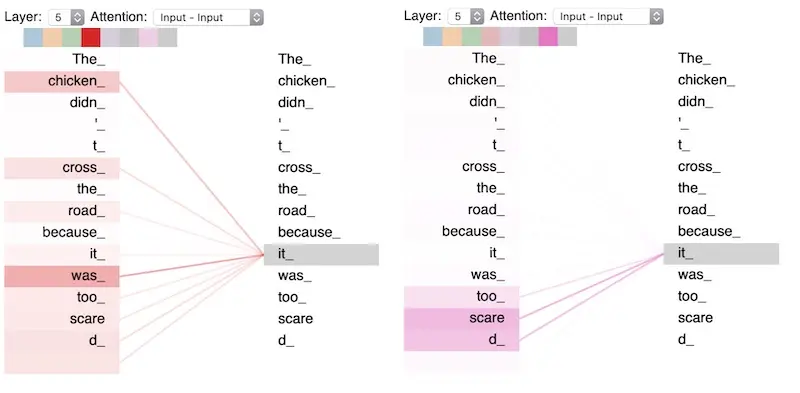
Why didn't the chicken cross the road? Attention from two different heads (source)
To provide information about the relative and absolute position of tokens in a sequence, positional encodings were used at the bottom of the encoder and decoder stacks. This helps the model to learn from token positions as well as the distance between each token.
(Be sure to check out Jay Alammar’s beautiful write-up on “The Illustrated Transformer”.)
Fine-tuning learned embeddings (2017)
So far, we’ve mostly used word embeddings directly, or concatenated them with input tokens (i.e., ELMo). There was no fine-tuning of the word embeddings for specific tasks. This changed with ULMFiT and OpenAI GPT (and transfer learning).
ULMFiT (2017) uses AWD-LSTM (LSTM with dropout at the various gates) as its language model and introduced a fine-tuning phase as part of three steps. First, in general-domain LM pre-training, the LM is trained on unlabelled data. ULMFiT trained on Wikitext-103 (28.6k Wikipedia articles and 103 million words).
Then, in target-task fine-tuning, the LM is fine-tuned with the corpus of the target task (no labelled data introduced yet). Discriminative fine-tuning is applied, where each layer is fine-tuned with different learning rates—the last layer has the highest learning rate, with each subsequent layer having reduced learning rates. ULMFiT also adopted slanted triangle learning rates where the learning rate increases quickly before decaying at a slower rate.
Finally, in target-task classifier fine-tuning, two additional linear blocks are added on the LM (softmax for the last layer, ReLU for the intermediate layer). Gradual unfreezing is done, where we start with unfreezing the last LM layer and fine-tuning it. One by one, each subsequent layer is unfrozen and tuned.
GPT (2017; granddaddy of GPT-3) also applied unsupervised pre-training. It uses the Transformer’s decoder stack. This is an improvement over LSTMs as the Transformer has better learning on long-ranged dependencies and is not recurrent in nature.
GPT is trained via two steps. First, unsupervised pre-training (similar to ULMFiT’s first step) involves learning on a corpus to predict the next word. GPT used the BookCorpus dataset of 7,000 unique, unpublished books. (This differs from ELMo, which uses shuffled sentences, thus destroying the long-range structure).
Then, supervised fine-tuning tweaks the decoder block for the target task. Task-specific inputs and labels are passed through the pre-trained decoder block to obtain the input representation (i.e., embedding). This representation is then fed into an additional linear output layer. In this stage, an auxiliary objective is included. The auxiliary objective predicts the next word in the task-specific corpus (similar to ULMFiT’s second step) and was found to improve generalisation and speed up convergence.
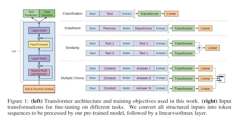
Inputs are transformed into a single sequence based on the task (source)
To use GPT, task-specific input transformations were done for various tasks:
- Text classification: The model can be used directly.
- Textual entailment: The premise and hypothesis is concatenated with a
$token. - Similarity: We get both orders of the sentences (i.e., sentence1-sentence2, sentence2-sentence1) and concatenate them. The decoder output is added element-wise and fed into a linear layer.
- Multiple-choice Q&A: Concatenate the question with each possible answer and feed them through a linear layer. The outputs are normalised via softmax to get a probability distribution.
(Check out Modern NLP’s Transfer Learning In NLP for comprehensive review on this.)
BERT: No recurrence, bidirectional, pre-trained (2018)
Towards the end of 2018, Bidirectional Encoder Representations from Transformers (BERT) was introduced. It obtained SOTA results on eleven NLP tasks. There were several elements from previous models that made BERT a pragmatic SOTA model:
- Transformer: BERT uses the Transformer encoder stack and does away with recurrence (parallelizable training).
- ELMo: Similar to ELMo, BERT has bidirectional context.
- ULMFiT and GPT: BERT also adopts pre-training and fine-tuning; thus, the LM (from pre-training) can be tuned for various downstream tasks.
- GPT: BERT also has a unified architecture and a single input representation.
BERT uses a multi-layer bidirectional Transformer encoder block as its language model. In contrast, GPT uses a unidirectional Transformer decoder block while ELMo uses twin, separate LSTMs.
Input to BERT is represented as a single sentence or a pair of sentences (e.g., question and answer). BERT uses WordPiece embeddings. It also introduces a special classification token (CLS) that is always the first token in a sequence—the final hidden state of this token is used for classification tasks. Sentence pairs are separated by a SEP token (similar to GPT).
Pre-training is done via two unsupervised tasks. First, a masked language model (LM) is trained via the cloze task. (The standard, predict-the-next-word task cannot be used with bidirectional context and multiple layers; more below). BERT masks 15% of tokens randomly (with the MASK token). However, this creates a mismatch between pre-training and fine-tuning. Thus, of the masked tokens, 80% are MASK, 10% are replaced by a random token, and 10% are unchanged. The LM predicts the original token with cross-entropy loss.
Why can’t we use bidirectional context with multiple layers?
Let’s examine “Today is a hellacious day for writing” with attention layers.
In the first layer, the vector for “hellacious” does not include itself. However, in layer two, the vector of the words around “hellacious” will include the vector for “hellacious” due to attention (the orange arrow). (In the example below, I only show the this for “day”.) Thus, from layer 3 onwards, the vector for “hellacious” will be able to see itself as part of the weighted attention in layer 2 (the red arrow).
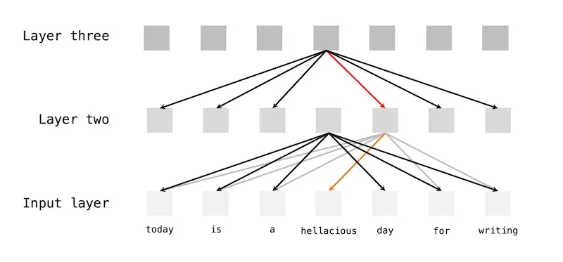
How tokens can see themselves via attention from lower layers
The second pre-training task involves next sentence prediction (NSP). Assuming two consecutive sentences A and B, 50% of the time sentence B actually follows sentence A. The other 50% of the time sentence B is a random sentence.
For both pre-training tasks, BERT uses the BooksCorpus (that GPT also used) and English Wikipedia (2,500 million words, text passages only). A document-level corpus was specifically chosen to learn from long contiguous sentences.
Fine-tuning involves passing task-specific inputs and labels to tweak model parameters end-to-end. Then, BERT can be used in various ways:
- Single sentence and sentence-pair classification: Use the final hidden state of
CLS - Single sentence tagging: Use the final hidden state of each token
- Q&A: Predict two probabilities per token, whether it’s the start or end of the text.
BERT is practical (read: lower cost and faster to train due to no recurrence) and high performing. As a result, it has been applied to Google Search.
More examples of machine learning applied in the real-world:
applied-ml
Ablation study: How does each BERT feature add to performance?
Ablation studies come from experimental neuropsychology, where parts of animals’ brains were removed to study the impact on their behaviour. In the context of machine learning, the term is used to describe removing certain parts of neural networks to gain a better understanding of the network behaviour.
Ablation studies are crucial for deep learning research -- can't stress this enough.
Understanding causality in your system is the most straightforward way to generate reliable knowledge (the goal of any research). And ablation is a very low-effort way to look into causality.
— François Chollet (@fchollet) June 29, 2018Findings from ablation studies on BERT:
- Removing next-sentence prediction reduced performance significantly.
- Without bidirectional language modelling (i.e., only left-to-right like in GPT), performance is reduced significantly.
- A larger model often leads to accuracy improvements, even when the labelled training samples are as few as 3,600.
- Using BERT for feature extraction (i.e., just using the word embeddings) also works well. The best approach is to concatenate the word representations from the top four hidden layers of the pre-trained encoder.
- While masked language modelling converges slower than left-to-right language modelling, masked language modelling eventually achieves higher accuracy with the same number of steps.
More details of the ablation studies in the BERT paper.
Improving on BERT (2019+)
Since BERT, several improvements have been made to make it lighter (DistilBERT, ALBERT), optimize it further (RoBERTa). BERT has also been applied to create sentence embeddings in 109 languages.
One problem BERT had was not being able to learn bidirectionally (which is why BERT used the cloze task for pre-training). XLNet (June 2019) addresses this via permutation language modelling (LM); in contrast, BERT used masked language modelling.
Permutation LM is tricky but here’s my attempt to explain it. Here’s our example sentence and token indices: “Today(1) is(2) a(3) hellacious(4) day(5) for(6) writing (7)”, with the sequence 1234567.
First, permutation LM creates multiple sequence permutations (e.g., 2347516). Then, it learns representations of each word based on only the preceding tokens: token 4 learns from tokens 2 & 3; token 7 leads from tokens 2, 3, 4. This ensures that the predicted word is never seen indirectly. (Note: This permutation is only used in the computation of attention; the order of tokens in the sequence is unchanged.)
BERT also had fixed-sized segments and thus could not handle sequences longer than the segment length (usually 512). XLNet uses previous work from Transformer-XL to get around this—it transfers state across fixed-sized segments (i.e., recurrence on segments) to handle sequences longer than the segment length. Nonetheless, with permutation LM and reintroducing recurrence, XLNet is much more computationally demanding to train.
Recently, Big Bird (28 July 2020) increased the segment length to 8x of what BERT could handle. BERT is limited by the quadratic dependency of its sequence length due to full attention, where each token has to attend to every other token. This leads to a memory limitation. On standard hardware (16gb RAM), this translates to input sequences (and segment length) of 512 tokens.
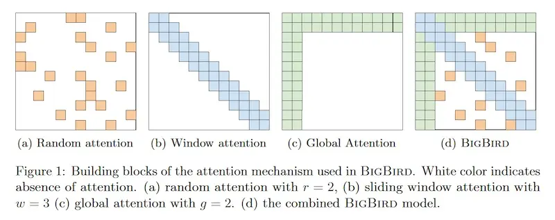
Big Bird has sparser attention that allows it to model on 8x the sequence length of BERT (source)
Big Bird proposed generalized attention mechanism which has linear complexity (as opposed to quadratic) on the sequence length. It has three aspects of attention:
- Random attention: Attends to
rrandom tokens, leading to sparse attention (r= 2). - Sliding window attention: Attends to a window of width
w(w= 3). This is similar to Longformer which uses a localised sliding window-based mask to reduce computation and extend BERT to longer sequences. - Global tokens: Global tokens are a subset of
gtokens in a sequence (g= 2). Global tokens attend to all tokens in the sequence and vice versa. This includes additional tokens such asCLSala BERT. (Using just random and sliding window attention were insufficient to compete with BERT).
Everything is text-to-text
Towards the end of 2019, the Text-To-Text-Transfer-Transformer (T5) introduced a unified framework that converts all text-based problems into a text-to-text format. Thus, the input and output are text-strings, making a single T5 fit for multiple tasks.
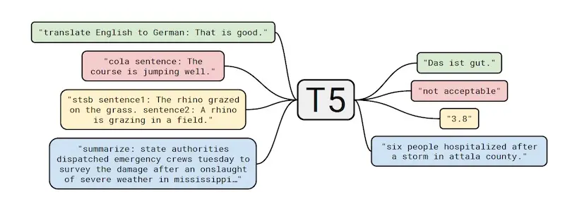
Translation, Q&A, classification are all text to text, with different prefixes to indicate the task (source)
The T5 uses the Transformer encoder-decoder based structure which the authors found to work best for text-to-text. Nonetheless, the authors introduced a few changes such as: removing the layer norm bias, placing the layer norm outside the residual path, and using a different position embedding scheme.
Pre-training was done on the Colossal Clean Crawled Corpus (C4), a high quality pre-processed English language corpus. It is approximately 750gb in size and is a cleaned version of the Common Crawl.
How did C4 come about?
C-4, or Composition C-4, was developed by the British during World War II … I’m kidding. (Well, while that is how the explosive was developed, it’s not the C4 we’re discussing here. Context is important.)
First, let’s start with the Common Crawl. The Common Crawl is a publicly available web archive of “web extracted text” from scraped HTML files. It produces 20TB fo data each month. But most of the text is not natural language—there’s a lot of gibberish, boilerplate, error messages, etc.
To clean Common Crawl (and get C4, a 750gb dataset), the following was done:
- Only retain lines ending with a terminal punctuation mark.
- Discarded pages with <5 sentences that only retained lines with >= 3 words.
- Removed pages with words on a “dirty, naughty, obscene, bad words” list.
- Excluded any line with the word
javascript. - Removed pages with
lorem ipsum. - Removed pages with
{to exclude pages containing code. - Deduplicated three-sentence spans occurring more than once in the data.
- Filtered out pages not classified as English with probability of >= 0.99.
With the unified format, the authors thoroughly explored the effectiveness of transfer learning in NLP. I loved how a sizeable portion of the paper was devoted to experiments (and “What didn’t work”) on architectures, objectives, fine-tuning approaches, etc. Here’s a high-level summary (reading the original paper is recommended):
- The encoder-decoder architecture with denoising objective worked best (vs. single Transformer stack, language modelling objective)
- Among the unsupervised objectives, masked language modelling (BERT-style) worked best (vs. prefix language modelling, deshuffling, etc.)
- There was limited difference between BERT-style objectives (e.g., replacing the entire corrupted span with a single
MASK, dropping corrupted tokens entirely) and different corruption probabilities (e.g., 10%, 15%, 25%) - Training on the full dataset for 1 epoch worked better than training on a smaller data set for multiple epochs (my view: more data > more compute)
- Fine-tuning all layers simultaneously performed best (vs. unfreezing each layer and tuning it, adding adapter layers of various sizes)
- Increasing model size had a bigger impact relative to increasing training time or batch size.
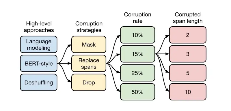
Hyperparameter tuning approach on unsupervised objectives for pre-training (source)
Downstream performance on a variety of benchmarks was evaluated (e.g., GLUE and SuperGLUE text classification, CNN/Daily Mail abstractive summarization, SQuAD question answering, and WMT translations.) With the insights from the experimental study, SOTA performance was achieved on 18 out of 24 tasks considered.
Summary
Whew, a lot has happened in NLP since 1985. To recap, here’s what we covered so far:
- Sequential models: RNN (1985), LSTM (1997), GRU (2014)
- Word embeddings: Word2vec (2013), GloVe (2014), FastText (2016)
- Word embeddings with context: ELMo (2018)
- Attention: Transformer (2017)
- Pre-training: ULMFiT (2017), GPT (2017)
- Combining the above: BERT (2018)
- Improving BERT: DistilBERT, ALBERT, RoBERTa, XLNet (2019); Big Bird, Multilingual embeddings (2020)
- Everything is text-to-text: T5 (2019)
And here’s a table summary if that’s what you prefer.
| Details | |
|---|---|
| RNN (1985) | Learns on sequences; hidden state of one time-step used as input to next time-step |
| LSTM (1997) | Adds gates (e.g., forget, input) to RNN; models long-range dependencies better |
| GRU (2014) | Simplifies LSTM and has lesser gates (i.e., update, reset); faster to train |
| Word2Vec (2013) | Unsupervised learning of word representations via CBOW and Skip-gram with sampling and negative subsampling |
| GloVe (2014) | Unsupervised learning of word representations via co-occurrence matrix |
| FastText (2016) | Unsupervised learning of word representations via character segments |
| ELMo (2018) | Unsupervised learning of word representations via bidirectional language model (two-layer LSTM); considers context of entire sentence |
| Transformer (2017) | Removes need for recurrence via attention and positional encodings; faster and less compute heavy to train |
| ULMFiT (2017) | Pre-training and fine-tuning on AWD-LSTM with discriminative fine-tuning, slanted triangle learning rates, and gradual unfreezing |
| GPT (2017) | Pre-training and fine-tuning on Transformer decoder stack; single input representation for various tasks |
| BERT (2018) | Pre-training and fine-tuning on Transformer encoder stack, bidirectional context via masked language modelling, single input representation |
| XLNet (2019) | Permutation language modelling, recurrence across fixed sized segments to handle longer sequences |
| T5 (2019) | Unified text-to-text format on Transformer encoder-decoder architecture and denoising objective, trained on C4 |
| Big Bird (2020) | Generalized attention mechanism to increase segment length to 8x of BERT |
Did I miss any key milestones? Let me know by responding to this tweet or in the comments below!
NLP is developing at a very fast pace.
— Eugene Yan (@eugeneyan) August 20, 2020
I recently took some time to review my notes and write a summary of the broad strokes (e.g., embeddings, architectures, transfer learning).
Did I miss anything important/oversimplify? Any error? Feedback welcome! https://t.co/264TycIQDf
References
- RNN: Serial Order: A Parallel Distributed Processing Approach
- LSTM: Long Short-Term Memory
- AWD-LSTM: Regularizing and Optimizing LSTM Language Models
- GRU: Learning Phrase Representations using RNN Encoder-Decoder for Statistical Machine Translation
- Word2vec: Efficient Estimation of Word Representations in Vector Space, Distributed Representations of Words and Phrases and their Compositionality
- GloVe: Global Vectors for Word Representation
- FastText: Enriching Word Vectors with Subword Information
- ELMo: Deep Contextualized Word Representations
- Transformer: Attention Is All You Need
- ULMFiT: Universal Language Model Fine-tuning for Text Classification
- GPT: Improving Language Understanding with Unsupervised Learning
- WordPiece embeddings: Google’s Neural Machine Translation System: Bridging the Gap between Human and Machine Translation
- BERT: Pre-training of Deep Bidirectional Transformers for Language Understanding
- DistilBERT: Smaller, Faster, Cheaper, Lighter; A Distilled Version of BERT
- ALBERT: A Lite BERT for Self-supervised Learning of Language Representations
- RoBERTa: A Robustly Optimized BERT Pretraining Approach
- Transformer-XL: Attentive Language Models Beyond a Fixed-Length Context
- Multilingual BERT embeddings: Language-agnostic BERT Sentence Embedding
- XLNet: Generalized Autoregressive Pretraining for Language Understanding
- Longformer: The Long-Document Transformer
- Big Bird: Transformers for Longer Sequences
- T5: Exploring the Limits of Transfer Learning with a Unified Text-to-Text Transformer
Thanks to Yang Xinyi and Pratik Bhavsar for reading drafts of this.
If you found this useful, please cite this write-up as:
Yan, Ziyou. (Aug 2020). NLP for Supervised Learning - A Brief Survey. eugeneyan.com. https://eugeneyan.com/writing/nlp-supervised-learning-survey/.
or
@article{yan2020nlp,
  title   = {NLP for Supervised Learning - A Brief Survey},
  author  = {Yan, Ziyou},
  journal = {eugeneyan.com},
  year    = {2020},
  month   = {Aug},
  url     = {https://eugeneyan.com/writing/nlp-supervised-learning-survey/}
}
Share on:
Browse related tags: [ llm deeplearning survey ] or
Join 11,800+ readers getting updates on machine learning, RecSys, LLMs, and engineering.